Stochastic Modeling in Biology
Introduction
Genetically engineered cells and organisms are being used to produce array of commonplace commercial products including drugs and materials. Biological engineering is being employed to enhance nutrition content of various foods and yield of crops. Recently, lab-grown meat represents an interesting alternative to traditional production and synthetic biology is being explored even by artists. These successes are, however, just baby steps in face of the richness and complexity of “products” nature is so adept in engineering. Like what you ask? Like YOU, for example.
In the meantime, development is ongoing at rapid pace. We are getting finer understanding of molecular-scale processes by which the life is implemented and by extension, we are becoming more adept in exercising control over them. Biology is becoming easier to analyze and design using established engineering approaches. At different system levels, from molecular to cellular to populational, mathematical modeling and abstraction in design are becoming possible. (If this abstraction thing is too abstract for you, think about this as if in your Arduino project (like this one) you had to build and debug the microcontroller first. Before you could do that, you would have to do the same for all the resistors, transistors and other elements of the board. Instead, and luckily, you just need to have the board shipped and plug it into your laptotp to boot it up. You don’t have to think of all the possibly very intricate details that make it work and can focus on building some application on top of it. This is the power of abstraction in design when put to work.).
This is exciting, fun and hugely relevant because, take it from Elon Musk Steve Jobs:
[…] the biggest innovations of the 21st century will be at the intersection of biology and technology.
Of course this topic is about as broad as an average statement of a politician so I will not try to cover it all here (If you are interested in some slightly more scientific peek into the topic, a good place to start is this video where Chris Voigt first gives general of the field and later explains his idea of programming genetic circuits the way we program computers), rather I want to focus on the mathematical modeling part. I find it really nice how this helps me to think about the biological process in more rigorous and engineering way and believe you may benefit from this as well.
First, I will give you lightweight introduction to some theory behind and then show some code I wrote for simulating simple transcription and translation processes. It is all on github so feel free to grab it afterwards to have some fun with it.
Biochemical Reaction Systems
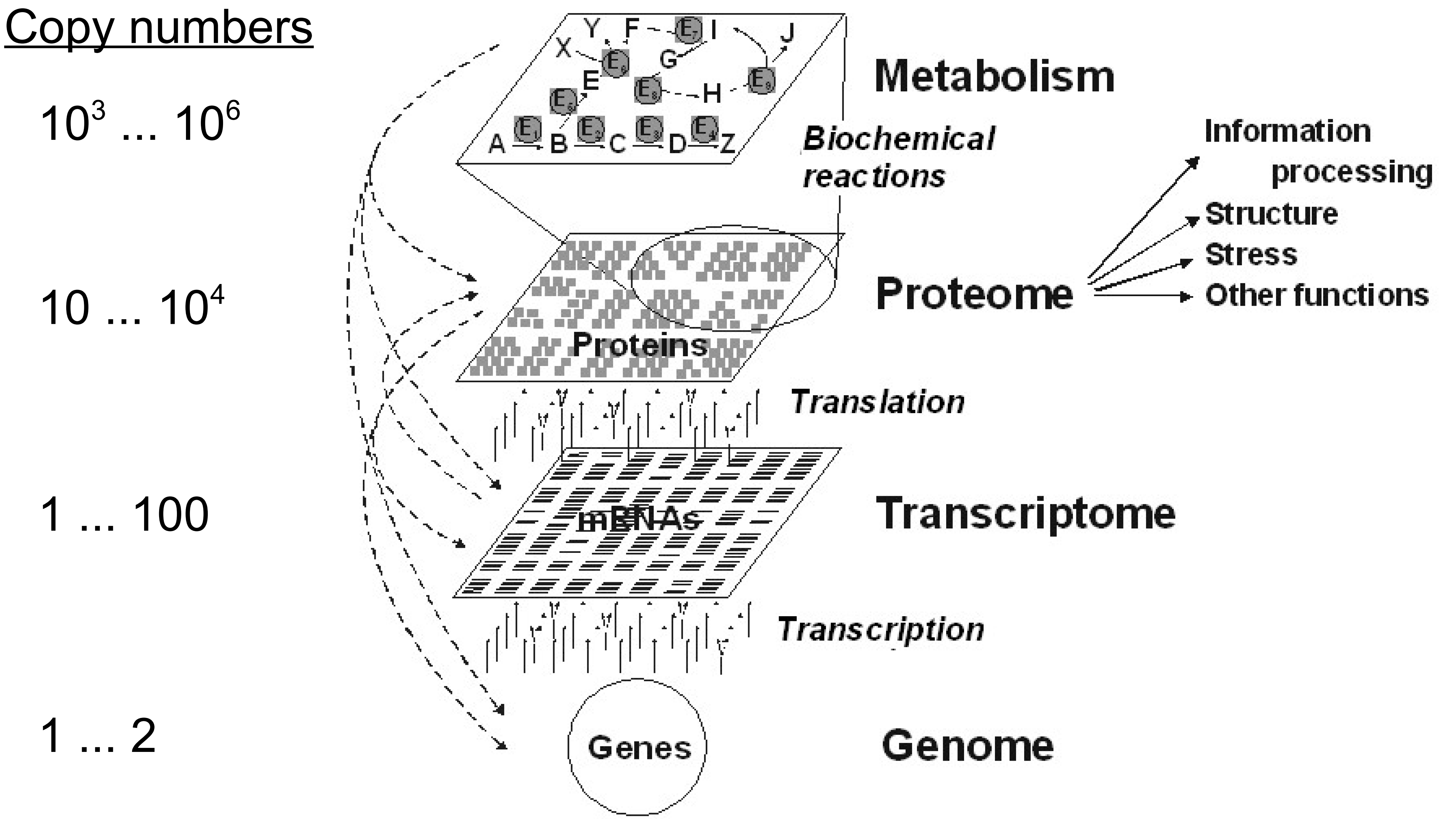
In what follows we are looking at distinct biochemical species present in a cell. Additionally, these species are present in low copy numbers that are significantly influenced by stochastic (random) events. You can think about this as having a big parking lot under your kitchen window (poor you) and not having a calendar. In the morning when you make your breakfast, you can very reliably say if it is a normal working day or a public holiday based on occupancy of the parking lot. Conversely, you friend, who has just two parking places within sight of his kitchen window cannot make a good guess of whether it is a public holiday or not based on if the two spots are empty. This could just as well be because somebody’s child got sick (which is as random event as it gets).
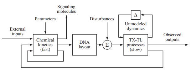
In biology, there are multiple sources of such randomness, including external environmental perturbations and inherent stochasticity stemming from statistical thermodynamics of molecular reactions. To account for this, we leave the familiar realm of concentrations and enter the world of single-molecule counts. In mathematical terms this means, that instead of writing differential equations for average concentration levels, we keep track of individual reaction events that have some probability of occurring on some time interval. Conceptually, the modeling framework is depicted in the following figure:
The Chemical Master Equation
We want to resolve dynamics of a system at very fine scale both in space and time. Further, the system does not have equilibrium configuration. It turns out that we are interested in probability $P(\mathbf{q}, t)$ of a system to be in microstate $\mathbf{q}$ at time $t$. Microstate is somewhat elusive term, but in the case of chemical reaction systems this is just a vector of number of molecules of each species in the system.
Next, we assume that there are $M$ reactions $R_j$, $j = 1, …, M$ in total and that $\boldsymbol{\nu}_j$ is a change in state (i.e. change in number of molecules, e.g. $\pm 1$ for unimolecular reaction) associated with reaction $R_j$. If we look at sufficiently small time interval, we can write $a_j (\mathbf{q})dt$ for the probability that a reaction $j$ “fires” in interval $dt$, given that current microstate of the system is $\mathbf{q}$. The $a_j (\mathbf{q})$ is called propensity function and we have dropped the time dependence as we assume this is accounted for by the dependence on microstate (that itself changes in time).
The above definitions allow us to calculate the change of the probability distribution function over an interval $dt$:
\[\begin{array}{lcl} P(\mathbf{q}, t + dt ~|~ \mathbf{q}_0, t_0) & = & P(\mathbf{q}, t ~|~ \mathbf{q}_0, t_0)\prod_{j=1}^{M}{(1-a_j(\mathbf{q})dt)} \\ & + & \prod_{j=1}^{M}{P(\mathbf{q} - \boldsymbol{\nu}_j, t ~|~\mathbf{q}_0, t_0)(a_j(\mathbf{q} -\boldsymbol{\nu}_j)dt)} \\ & = & P(\mathbf{q}, t ~|~ \mathbf{q}_0, t_0) \\ & + & \sum_{j=1}^{M}{\bigg(P(\mathbf{q} - \boldsymbol{\nu}_j, t ~|~\mathbf{q}_0, t_0)a_j(\mathbf{q} -\boldsymbol{\nu}_j) - P(\mathbf{q}, t ~|~ \mathbf{q}_0, t_0)a_j(\mathbf{q})\bigg)dt} \\ & + & \mathscr{O}(dt^{2})\\ \end{array}\]This may look scary but it really just states that the probability to get to state $\mathbf{q}$ is equal to probability that we are already in that state + the probability that we are one reaction away from that state and the matching reaction fires in the interval $dt$. After dropping higher order terms in $dt$ and simplifying the notation we get:
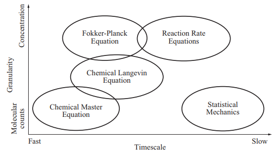
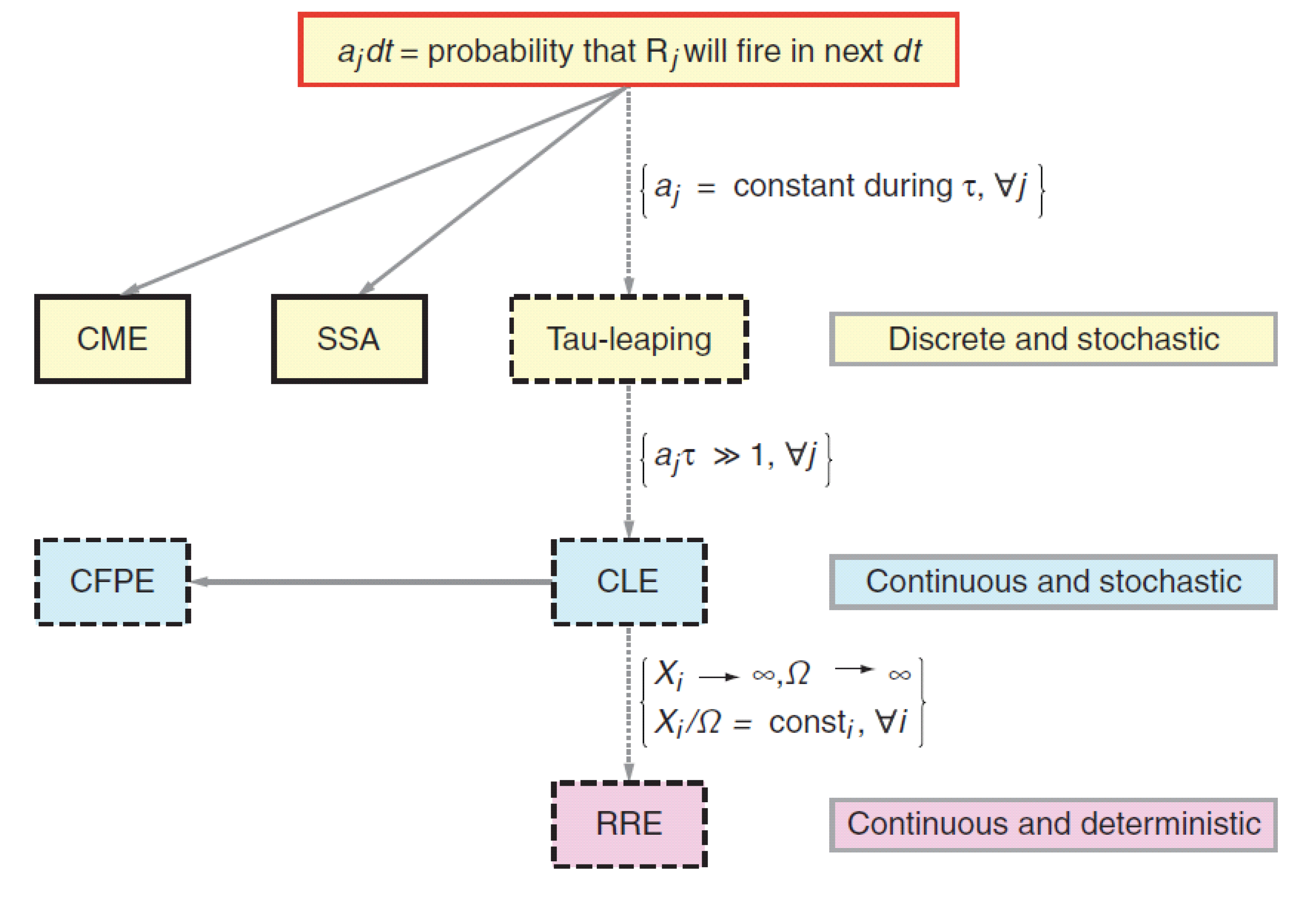
\[\frac{\partial P}{\partial t} (\mathbf{q}, t) = \sum_{j=1}^{M}{\bigg(P(\mathbf{q} - \boldsymbol{\nu}_j, t)a_j(\mathbf{q} -\boldsymbol{\nu}_j) - P(\mathbf{q}, t)a_j(\mathbf{q})\bigg)}.\]This is the chemical master equation (CME), which is an example of forward Kolmogorov equation for a discrete state, continuous time random process (phew, quite some terminology here). The discrete state here is described by the vector $\mathbf{q}$ with numbers of molecules of species in the system. To be able to calculate anything with it we will need to specify the initial condition $P(\mathbf{q}_0, t_0)$. To help you put this into bigger picture, see the two following figures that show where the CME is positioned with respect to other (more approximate) approaches to model biological system dynamics.
The main reason for why there is such a wide palette of approaches is because the chemical master equation does not have analytical solution and its numerical solution quickly becomes computationally expensive for systems with more than few distinct species. Its advantage is that building a model from set of reactions is very transparent and straightforward and this is why we will focus on precisely this approach, keeping in mind its limitations.
The Stochastic Simulation Algorithm
We have already mentioned that CME doesn’t have analytical soltion. The straightforward approach how to obtain some representative description of the system is to draw samples from the probability distribution $P(\mathbf{q}, t ~|~ \mathbf{q}_0, t_0)$ governed by the CME. This is Monte Carlo simulation. We will be able to determine moments of the distribution (e.g. mean and variance) by averaging over many independent realizations of single trajectories (under identical initial conditions).
State update
To implement this in code, we will follow approach as developed by Daniel Gillespie, i.e. the stochastic simulation algorithm (SSA). Given an arbitrary state $\mathbf{q} = (n_1, n_2, …)$, for computation of the next state we need an index of next reaction that occurs (“fires”) and $\Delta t$ in which this happens. The probability that the next reaction to fire is the reaction $j$ is directly proportional to the corresponding propensity $a_j$ (intuitively, reactions with high reaction rates will occur more often). Therefore finding an index $j$ of such reaction is just matter of drawing a random integer from a weighted distribution on $[1, M]$ where the weights are given as:
Note that this is equivalent to drawing a uniform random number on $[0,1]$, scaling it by the total propensity $a = \sum_{i}^{M}a_i$ and finding the first integer $j$ for which this scaled random number is less then $\sum_{i}^{j}a_i$.
Time update
Finding a $\Delta t$ in which this reaction occurs is more involved. You can find the derivation at the end of this post, but for now we will take for granted that the cumulative distribution function (CDF) for $\Delta t$ is:
This is nice because we draw samples from this distribution by drawing a random number $\xi$ on $[0, 1]$ and inverse-sampling from the CDF. In this case, the CDF can be even inverted analytically to obtain:
\[\Delta t = \frac{1}{a} \mathrm{ln}\bigg(\frac{1}{1 - \xi}\bigg).\]Python code
If the previous two sections sounded complicated to you, have no worry, it is actually dead simple to implement them in code:
def draw_ssa(propensities, total_prop):
    """Draw random samples according to prescriptions of SSA

    Parameters
    -------
    propensities: array, propensities of all reactions
    total_prop: float, total propensity

    Returns
    ---------
    idx: int, index into the state change matrix to determine updated
              state
    tau: float, time step size
    """

    xi1 = np.random.uniform(0,1)
    prop_rank = np.sort(np.cumsum(propensities)/total_prop)
    idx = np.int32(np.argmax(prop_rank > xi1))

    xi2 =  np.random.uniform(0,1)
    tau = np.float32(1/total_prop * np.log(1/(1-xi2)))
    return idx, tau
The Algorithm
Now we are armed for the stochastic simulation algorithm that proceeds as follows:
This algorithm is also called Gillespie’s direct method as it was D.T. Gillespie who proved that this method samples from the probability distribution governed by the CME. The method is derived based on first principles. This makes it an exact approach to stochastic simulation, consequently, time step $\tau$ is not mere finite approximation (as in ODE models).
Python code
Implementation in code is again quite simple:
def ssa_routine(k, t_end, q0, nu, psi):
    """ Stochastic Simulation Algorithm

    Performs sampling from distribution governed by chemical master equation.

    Parameters
    --------------
    k: array, vector stochastic reaction constants
    t_end: int, number of steps for the simulation
    q0: array, initial number of molecules for each species
    nu: ndarray, stoichiometric matrix, with state change vectors in columns
    psi: ndarray, reactant molecularity matrix

    Returns
    --------------
    Q: array, all states q at times t
    time: array, vector of times t
    tot_props: array, total propensities at times t
    is_success: bool, flag indicating if simulation ran to completion
    """

    #Initialize arrays to store states, tick times
    time = []
    t = 0
    time.append(t)

    Q = []
    state = q0
    Q.append(state)

    while t < t_end:
        # Calculate propensities for current state
        propensities, total_prop = get_propensities(k, state, psi)

        # Draw random samples for update of state and time step
        idx, tau = draw_ssa(propensities, total_prop)

        ## Find random change in state - see theory
        state = state + nu[idx, :]

        ## Find random time step size - see theory
        t = t + tau

    return Q, time
def get_propensities(rates, populations, psi):
    """Return propensities given rates and populations

    Computes the value of propensity for all reactions. Generalizes to various systems

    Parameters
    ----------
    rates: array, vector of stochastic reaction constants
    populations: array, vector of number of molecules of each species

    Returns
    ---------------
    propensities: array, vector of propensiites for all reactions
    total_propensity: float, sum of all propensiites
    """

    # See model description
    propensities = np.empty(psi.shape[0], dtype = np.float32)
    for r in range(psi.shape[0]):
        temp = populations ** psi[r,:]
        propensities[r] = temp.prod() * rates[r]

    total_propensity = np.float32(propensities.sum())

    return propensities, total_propensity
The apparent drawback of this method is its computational complexity. As the systems become of somewhat more practical size (larger number of different species), the time step becomes very small (reactions occur often). As on each time step, two random numbers have to be generated, this leads to significant computational cost. To circumvent this issue, approximations of the SSA become useful (see Figure Hierarchy of methods for modeling biochemical reactions).
Easy example: The Central Dogma
To make this discussion more concrete, let’s look at the minimal example of central dogma of molecular biology. This can be concisely represented as:
Here the microstate is simply the vector $\mathbf{q} = (1, n_m, n_p)$, where $n_m$ and $n_p$ are the copy numbers of transcripts and proteins respectively that depend on time. The DNA is present in single copy throughout (as such, we do not need to include it in our calculations, but will do so for consistency). The propensities (or transition probabilities) are:
\[a_1 = \beta_m \qquad a_2 = \gamma_m \cdot n_m \qquad a_3 = \beta_p \cdot n_m \qquad a_4 = \gamma_p \cdot n_p,\]where $\beta_i$ corresponds to production and $\gamma_i$ to degradation. We can see that propensity, in case of unimolecular reaction ($A \rightarrow B$) directly corresponds to the reaction rate constant (Things get only bit more complicated for bimolecular reactions as you will see later).
Each state change vector corresponds to one reaction in the system and together they are concatenated as columns of stoichiometric matrix $\mathbf{N}$:
\[\mathbf{N}= (\boldsymbol{\nu}_1^T, \boldsymbol{\nu}_2^T, \boldsymbol{\nu}_3^T, \boldsymbol{\nu}_4^T) = \begin{bmatrix} 0 & 0 & ~0 & ~0 \\ 1 & 0 & -1 & ~0 \\ 0 & 1 & ~0 & -1 \end{bmatrix}\]The dynamics of the system are described by Chemical master equation (CME) for probability $P\big((n_m, n_p), t\big)$:
\[\begin{array}{lcl} \frac{\partial P}{\partial t}\big((n_m, n_p), t\big) & = & P\big((n_m-1, n_p\big), t)\beta_m - P\big((n_m, n_p), t\big)\beta_m \\ & + & P\big((n_m+1, n_p), t\big)\gamma_m (n_m+1) - P\big((n_m, n_p), t\big)\gamma_m n_m \\ & + & P\big((n_m, n_p-1), t\big)\beta_p (n_m) - P\big((n_m, n_p), t\big)\beta_p n_m \\ & + & P\big((n_m, n_p+1), t\big)\gamma_p (n_p+1) - P\big((n_m, n_p), t\big)\gamma_p n_p \\ \end{array}\]Phew! This has been quite some theory we have covered, let’s now take a look how we can translate all this into code to simulate a real biological system.
Simulation
%load_ext autoreload
%autoreload 2
import ssa_routine as ssa
import numpy as np
import matplotlib.pyplot as plt

plt.style.use('ggplot') # use "ggplot" style for graphs
pltparams = {'legend.fontsize':14,'axes.labelsize':18,'axes.titlesize':18,
             'xtick.labelsize':12,'ytick.labelsize':12,'figure.figsize':(7.5,7.5),}
plt.rcParams.update(pltparams)
Model Parameters
We set the initial conditions as following:
| $DNA$ | $mRNAs$ | $Proteins$ |
|---|---|---|
| 1 | 0 | 0 |
For the reaction rates we select:
| $\beta_m$ | $\beta_p$ | $\gamma_m$ | $\gamma_p$ |
|---|---|---|---|
| 10 | 10 | 1 | 0.4 |
This means, for example, that the “birth” of a molecule of mRNA is 10-times more likely than its “death”.
Additionally we define matrix of reactant (species entering each reaction) molecularity $\mathbf{\psi}$:
\[\mathbf{\psi}= \begin{bmatrix} 1 & 0 & 0 & 0 \\ 0 & 1 & 1 & 0 \\ 0 & 0 & 0 & 1 \end{bmatrix}.\]We will also simulate multiple independent evolutions (paths) such that we can obtain mean evolution.
mp = ssa.modelParameters(k = np.array([10, 10, 1, .4]),
                         nu = np.array(([0, 1, 0], [0, 0, 1], [0,-1, 0], [0, 0,-1])),
                         psi = np.array(([1, 0, 0], [0, 1, 0], [0, 1, 0], [0, 0, 1])),
                         q0 = np.array([1,0, 0]),
                         t_end = 100,
                         names = ["gene", "mRNA", "protein"],
                         dist = ["none", "poiss", "gauss"] )
n_paths = 30
np.random.seed(123)
ssa.main(mp, n_paths, do_load = 0, do_save = 0)
2018-04-15 09:33:39,299:ssa_routine:INFO: Starting simulation with n_paths=30
2018-04-15 09:34:14,563:ssa_routine:INFO: Calculating statistics for all species.
2018-04-15 09:34:15,376:ssa_routine:INFO: Simulation finished.
2018-04-15 09:34:21,556:ssa_routine:INFO: Program execution finished.
| mean | var | CV | |
|---|---|---|---|
| gene | 1.000000 | 0.000000 | 0.000000 |
| mRNA | 10.431053 | 10.262420 | 0.307112 |
| protein | 252.870719 | 2027.642923 | 0.178073 |
Results
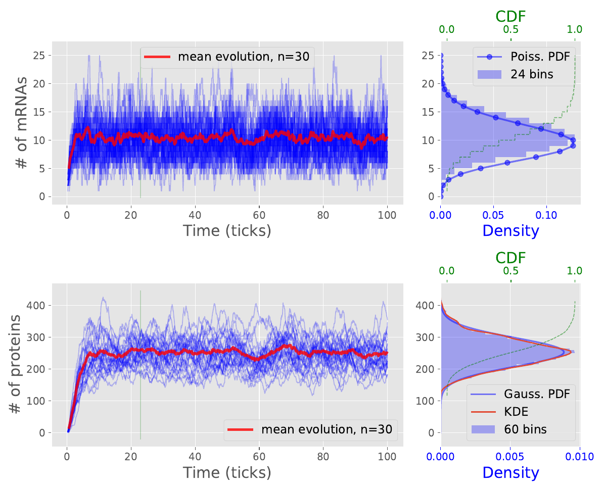
We obtain statistics for distribution of number of species. The mRNAs reach steady-state value of around 10 copies whereas the proteins level off at around 260 copies. The $CV$ is a coefficient of variation, normalized measure of dispersion of a distribution defined as a ratio of standard deviation to mean $CV = \frac{\sigma}{\mu}.$
We can look at the development of species numbers in time in the following plot in the left panel. On the right hand is then all-time histogram estimate of distribution of copy numbers together with empirical cumulative distribution function and KDE - kernel density estimate. We observe that the distribution of number of mRNAs well follows the theoretical Poisson distribution with rate parameter $\lambda = \beta_m$.
Note on speed
Even in this simple version, the algorithm takes quite some time to finish. I looked into it and improved the performance using numba. You can find details on this in the supplementary note.
Advanced Example: Noise Induced Switch
OK, once we have the simulation and visualization functions ready and once we can draw samples reasonably fast, we can start working on a more complex model. We will look at set of reactions that will allow us to simulate effects of noise on gene expression levels. In particular we are interested in rapid switching between two significantly different levels of expression. This interesting phenomenon, referred as bistability, is often present in real biological circuits but cannot be captured by a deterministic ODE model. Whereas in previous easy example we may have as well used a deterministic ODE to obtain good estimate of time evolution, in this case we need a stochastic model to get representative picture of system dynamics.
The model
\(G_1 \xrightarrow{\beta_1} G_1 + P_1 \qquad \qquad P_1 \xrightarrow{\gamma_1} \varnothing \tag{1a, 1b}\)
-
Reactions $(1a)$ and $(2a)$ represent expression of proteins $P_1$ and $P_2$ originating from genes $G_1$ and $G_2$ ($G_2$ codes for bicistronic mRNA). They reflect the fact that the genes are left unchanged and available for transcription.
-
$(2a)$ and $(2b)$ correspond to protein degradation, where reaction rate is proportional to current number of molecules of given protein $n_i, ~ i={P_1, P_2}$.
-
In equation $(3)$, the expression of protein $P_1$ is inhibited by $P_2$ which binds to promoter region of $G_1$ and acts as inhibitor, forming complex $\xi_1^I$.
-
The expression of from gene $G_2$ is repressed by protein $P_1$ which together form an intermediate transcription-inhibiting complex $\xi_2^{I_1}$ (reaction $(4)$)
-
Protein $P_1$ is inactivated by binding to complex $\xi_2^{I_1}$ and forming $\xi_2^{I_2}$ (reaction $(5)$). Note that reactions $(4)$ and $(5)$ work antagonistically.
We will model cooperativity of the enzyme binding sites with:
\[\kappa_{c3}^{+} = \sigma \kappa_{c2}^{+} \qquad \sigma >> 1.\]This essentially says that the inhibitory binding to $P_1$ becomes easier after the first complexation reaction. This, at the first sight not very interesting feature of the system, is actually essential in our simulation. Repression with cooperativity is namely one of ways how to achieve switch-like behavior in biological systems.
The system in question has 7 distinct biochemical species: $[G_1, P_1, G_2, P_2, \xi_{1}^{I}, \xi_{2}^{I_1}, \xi_{2}^{I_2}]$ and comprises of in total 10 reactions (as we consider each reversible reaction as two).
Stochastic reaction constants
As previously we will define an array of stochastic reaction rates $k$. We will have to be careful about units here. First, we note that for unimolecular reactions, the reaction rates are identical to the deterministic ones with unit ${min}^{-1}$. This is good because we are already familiar with them from previous example.
For bimolecular (two species) reactions, the stochastic reaction rate relates to the reaction rate of deterministic model by scaling with inverse volume $\Omega$.
\[\hat{k}_i = \frac{k_i}{\Omega}.\]To obtain same units as in the case of unimolecular reaction, we include also scaling by Avogardo’s number $N_A [mol^{-1}]$, such that $\Omega = V\, N_A$ and $k_i = [M \cdot min^{-1}]$. $N_A$ is the old familiar $6.022\cdot10^{23} mol^{-1}.$ For the volume, we make a ballpark estimate for E.coli as a cylinder with diameter $1\mu m$ and length $2\mu m$ yielding $V \approx 1.5 \mu m^3 = 1.5\cdot 10^{-14} dm^3$.
For our model, we will select the following values of stochastic reaction constants:
| $\beta_1$ | $\beta_2$ | $\gamma_1$ | $\gamma_2$ | $\kappa_{c1}^{+}$ | $\kappa_{c1}^{-}$ | $\kappa_{c2}^{+} $ | $\kappa_{c2}^{-}$ | $\kappa_{c3}^{+}$ | $\kappa_{c3}^{-}$ |
|---|---|---|---|---|---|---|---|---|---|
| $100$ | $1000$ | $10$ | $4$ | $\frac{2}{\Omega}$ | $1$ | $\frac{4}{\Omega}$ | $1$ | $\frac{4\sigma}{\Omega}$ | $1$ |
The choice here is less arbitrary then it may look, because only certain parameters of the system will lead to noise-induced switch-like behavior. Here we require $\kappa_{c1}^{-} = \kappa_{c2}^{-} = \kappa_{c3}^{-}$, $2 \kappa_{c1}^{+} = \kappa_{c2}^{+}$ and $\sigma = 10$.
This leads to following set of propensities:
| $a_1$ | $a_2$ | $a_3$ | $a_4$ | $a_5$ | $a_6$ | $a_7$ | $a_8$ | $a_9$ | $a_{10}$ |
|---|---|---|---|---|---|---|---|---|---|
| $\beta_1~n_{G1}$ | $\beta_2~n_{G2}$ | $\gamma_1~n_{P_1}$ | $\gamma_2~n_{P_2}$ | $\kappa_{c1}^{+}n_{P2}n_{G1}$ | $\kappa_{c1}^{-}~\xi_{1}^{I}$ | $\kappa_{c2}^{+}n_{P1}n_{G2}$ | $\kappa_{c2}^{-}~\xi_{2}^{I_1}$ | $\kappa_{c3}^{+}n_{P1}\xi_{2}^{I_1}$ | $\kappa_{c3}^{-}~\xi_{2}^{I_2}$ |
As previously we assume, that DNA does not degrade, although the transcription from it can be inhibited by binding with respective protein (reactions $3$ and $4$).
Further we set the initial conditions as following:
| $G_1$ | $P_1$ | $G_2$ | $P_2$ | $\xi_{1}^{I}$ | $\xi_{2}^{I_1}$ | $\xi_{2}^{I_2}$ |
|---|---|---|---|---|---|---|
| 1 | 10 | 1 | 10 | 0 | 0 | 0 |
Simulation
As the code in previous example was written with to be generalizable, we will be able to almost entirely reuse it, we just need to update the model parameters as follows:
# Model Parameters
sigma = 10
V = 1.5e-14
to_nanomolar = 1e-9
omega = 6.02214086e23*V*to_nanomolar
t_end = 30000
k = np.asarray([100, 1000, 10, 4, 2/omega, 1, 4/omega, 1, 4*sigma/omega, 1])
q0 = np.array([  1, 10,1, 10, 0, 0, 0])
names = [r'$G_1$', r'$P_1$', r'$G_2$', r'$P_2$',
         r'$\xi_1^{I}$', r'$\xi_2^{I_1}$', r'$\xi_2^{I_2}$']
dist = ["none"]*7
## State change matrix associated with each reaction
nu = np.array([ [0, 1, 0, 0, 0, 0, 0], #G1    -> G1+P1
                [0, 0, 0, 2, 0, 0, 0], #G2    -> G2+P2
                [0,-1, 0, 0, 0, 0, 0], #P1    -> _
                [0, 0, 0,-1, 0, 0, 0], #P2    -> _
                [-1,0, 0,-1, 1, 0, 0], #G1+P2 -> C1
                [1, 0, 0, 1,-1, 0, 0], #C1    -> G1+P2
                [0,-1,-1, 0, 0, 1, 0], #P1+G2 -> C2a
                [0, 1, 1, 0, 0,-1, 0], #C2a   -> P1+G2
                [0,-1, 0, 0, 0,-1, 1], #P1+C2a-> C2b
                [0, 1, 0, 0, 0, 1,-1]  #C2b   -> P1+C2a
              ], dtype = np.int)
## Molecularity of species entering each reaction
psi = np.array([[1, 0, 0, 0, 0, 0, 0],
                [0, 0, 1, 0, 0, 0, 0],
                [0, 1, 0, 0, 0, 0, 0],
                [0, 0, 0, 1, 0, 0, 0],
                [1, 0, 0, 1, 0, 0, 0],
                [0, 0, 0, 0, 1, 0, 0],
                [0, 1, 1, 0, 0, 0, 0],
                [0, 0, 0, 0, 0, 1, 0],
                [0, 1, 0, 0, 0, 1, 0],
                [0, 0, 0, 0, 0, 0, 1]], dtype = np.int)

mp_toggle = ssa.modelParameters(k, nu, psi, q0, t_end, names, dist)

#Simulation Parameters
n_paths = 1
do_load = 0 # default 0
do_save = 1 # default 1
np.random.seed(123)
ssa.main(mp_toggle, n_paths, do_load ,do_save)
2018-04-15 09:43:40,516:ssa_routine:INFO: Starting simulation with n_paths=1
2018-04-15 09:43:40,524:ssa_routine:INFO: Start of simulation for path # 1 out of 1.
2018-04-15 09:45:07,171:ssa_routine:INFO: Relative time: 0.20.
2018-04-15 09:46:01,920:ssa_routine:INFO: Relative time: 0.40.
2018-04-15 09:48:00,145:ssa_routine:INFO: Relative time: 0.60.
2018-04-15 09:49:25,028:ssa_routine:INFO: Relative time: 0.80.
2018-04-15 09:52:52,343:ssa_routine:INFO: Data saved to file results~/data/out_20180415-095212.
2018-04-15 09:52:52,605:ssa_routine:INFO: Calculating statistics for all species.
2018-04-15 09:53:29,373:ssa_routine:INFO: Simulation finished.
2018-04-15 09:54:03,614:ssa_routine:INFO: Program execution finished.
| mean | var | CV | |
|---|---|---|---|
| $G_1$ | 0.678624 | 0.218094 | 0.688165 |
| $P_1$ | 7.137714 | 31.071102 | 0.780943 |
| $G_2$ | 0.320242 | 0.217687 | 1.456927 |
| $P_2$ | 159.794211 | 54399.408869 | 1.459607 |
| $\xi_1^{I}$ | 0.321376 | 0.218094 | 1.453140 |
| $\xi_2^{I_1}$ | 0.005893 | 0.005858 | 12.988131 |
| $\xi_2^{I_2}$ | 0.673865 | 0.219771 | 0.695685 |
Results
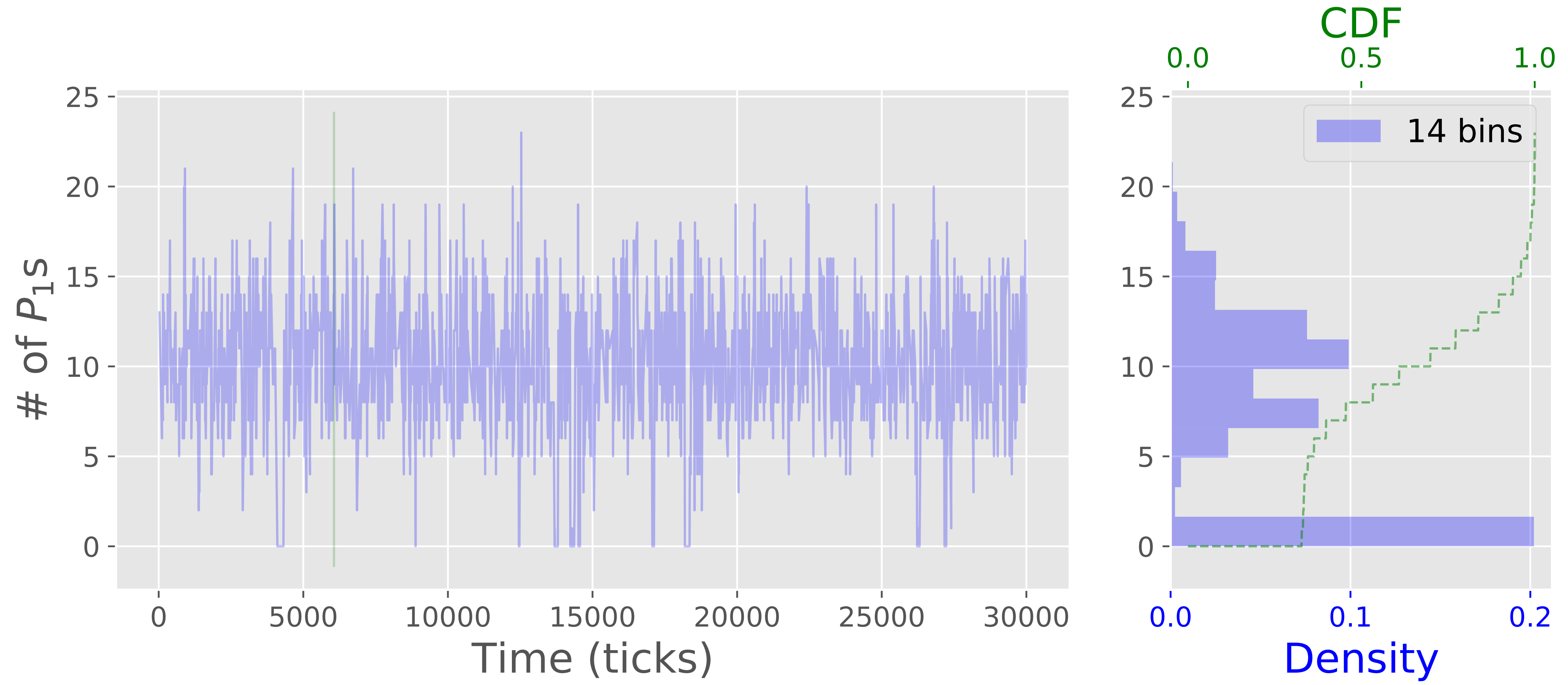
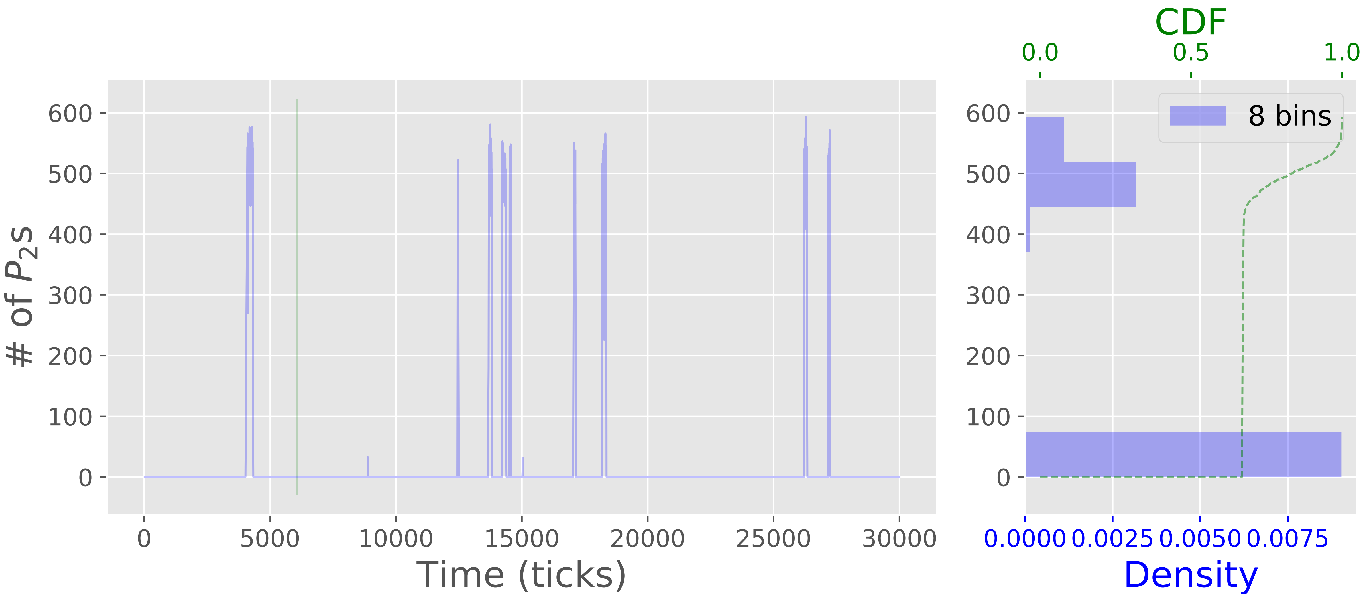
From the statistics, we may conclude that there is not much going on in our system, but look at the following plots of temporal evolution of protein copy numbers is more interesting. We see that the system manifests bistability when there are significant and abrupt jumps in copy numbers of both proteins. This is the expected effect of noise-induced switching that is not tractable in deterministic model. The bistable behavior is due to the fact that the copy numbers of the proteins are dependent on presence or absence of complexes $\xi_1^{I}$, $\xi_2^{I_1}$, $\xi_2^{I_2}$ that in turn acquire copy numbers only in set $\{0,1\}$. Such binary state is significantly affected by stochastic events (recall the previous example with parking lot).
Conclusion
If you have made it all the way here, pat yourself on the back. It has been quite some math we have covered and it allows you to faithfully simulate dynamical systems as intriguing and complicated as genetic circuits. Now you know something about the phenomenon of bistability, which is a crucial element of building a toggle-switch, one of the elemental parts in synthetic-biology. You also understand the important role of noise in gene expression and that the inherent stochasticity is not purely a complication in our design but can be efficiently exploited to drive patterns in molecular ‘decision-making’. In addition to Stochastic Simulation Algorithm, you are now also aware of other, more approximate, approaches for modeling biochemical (or other stochastic) systems like Chemical Langevin or Fokker-Planck equations that can allow you to inspect systems of larger size.
Last but not least, after inspecting the code in the github repository, you will have seen examples of some advanced python capabilities including function decorators, just-in-time compilation and logging.
I hope reading this post was as enjoyable for you as much as it was for me to write it. If you feel like you want to find more about the exciting field of synthetic biology, you can start with this video. In any case, stay tuned for upcoming posts on cool interdisciplinary and engineering topics.
Suplementary Notes
Time step size derivation for SSA
Define $p(\tau, j |\mathbf{q}, t)d\tau$ as the probability that the reaction $j$ occurs in the time interval $[t + \tau, t + \tau + d\tau]$, then we have:
\[p(\tau, j ~|~ \mathbf{q}, t)d\tau = P_0 (\tau ~|~ \mathbf{q}, t) \cdot a_j(\mathbf{q})d\tau,\]where $P_0 (\tau ~|~ \mathbf{q}, t)$ is the probability that no reaction fires on time interval $[t, \tau + t]$. We note that starting time $t$ is arbitrary and we may set it to zero. Corresponding probability that no reaction occurs in time interval $[t + \tau, t + \tau + d\tau]$:
\[P_0 (\tau + d\tau\ |\ \mathbf{q}, t) = P_0 (\tau\ |\ \mathbf{q}, t) \cdot (1-ad\tau),\]where $a = \sum_{i}^{M}a_i.$
It then immediately follows that:
\[\frac{d P_0}{d \tau} (\tau\ |\ \mathbf{q}, t) = -P_0 (\tau\ |\ \mathbf{q}, t) \cdot a.\]Solving this differential equation with initial condition $P_0 (0\ | \mathbf{q}, t) = 1$ yields:
\[P_0 (\tau\ | \mathbf{q}, t) = \mathrm{exp}(-a\tau).\]Going back to previous definition, this gives us:
\[p(\tau, j\ |\ \mathbf{q}, t) = \mathrm{exp}(-a\tau) \cdot a_j(\mathbf{q}).\]To obtain index of next reaction $j$ we marginalize over all $\tau$ and obtain:
\[\int_{0}^{\infty}p(\tau, j\ |\ \mathbf{q}, t) d\tau = a_j(\mathbf{q}) \int_{0}^{\infty} \mathrm{exp}(-a\tau)d\tau = \frac{a_j(\mathbf{q})}{a}.\]Similarly, to find time that next reaction occurs, we integrate over all reactions $j$ and obtain:
\[p(\tau\ |\ \mathbf{q}, t) = \mathrm{exp}(-a\tau) \cdot a.\]The probability that the reaction occurs on time interval $[0, \Delta t]$ is then given by the cumulative distribution function (CDF):
\[\int_{0}^{\Delta t}p(\tau\ | \mathbf{q}, t) d\tau = a \int_{0}^{\Delta t} \mathrm{exp}(-a\tau)d\tau = 1 - \mathrm{exp}(-a\Delta t).\]The CDF is bounded on $[0, 1]$ and we can easily generate samples from corresponding PDF by inverse-sampling when we draw uniformly distributed numbers $\xi$ which finally yields:
\[\Delta t = \frac{1}{a} \mathrm{ln}\bigg(\frac{1}{1 - \xi}\bigg),\]as stated before.
Optimizing the sampling in SSA
The computational burden of the direct method for SSA hits us pretty early. This can be troubling as it prolongs development cycles and limits number of species we can track. To alleviate this at least marginally, we can try to speed up our current code without making any conceptual changes to what is being computed and how (in contrast to more approximate approaches like Chemical Langevin Equation(CLE) and Fokker-Planck Equation (FPE)).
Use profiler to find where the most time is spent
First, we profile our code to see where the most time is being spend.
%load_ext line_profiler
import ssa_routine as ssa
import os
%lprun -T profiler.out -f ssa.ssa_routine ssa.ssa_routine(mp.k, mp.t_end, mp.q0, mp.nu, mp.psi)
\*\*\* Profile printout saved to text file 'profiler.out'.

Timer unit: 4.46227e-07 s
Total time: 3.26368 s
Function: ssa_routine at line 92

Line #      Hits         Time  Per Hit   % Time  Line Contents
==============================================================
    92                                           def ssa_routine(k, t_end, q0, nu):

    119     20580        71930      3.5      1.0      while t < t_end:
    120     20579      2325960    113.0     31.8          propensities, total_prop = get_propensities(k, state)

    125                                                   # Draw random samples for update of state and time step
    126     20579      3574266    173.7     48.9          idx, tau = draw_ssa(propensities, total_prop)

    141         1            3      3.0      0.0      return Q, time
Use numba to speed up the calculations
We have found out that absolute majority of the time is spent in computing propensities and drawing samples for update with a respective reaction in given time interval. Unsurprisingly, as these occur on each and every time-step. Clearly, we can get the most ‘bang for the buck’ by making these two steps faster. To this end, we place them into individual functions and use numba’s @jit decorator for just-in-time (JIT) compilation. This allows us to get about five-fold speed-up in calculations which I think is fair given the simplicity of implementation. This boils down to decorating the function as:
@numba.jit(nopython = True)
def some_function(x, y):
    return x + y
Here is the speed comparison:
%set_env NUMBA_DISABLE_JIT=1
#os.environ["NUMBA_DISABLE_JIT"] = "1"
%timeit -n 1 -r 3 ssa.simulate(mp, n_paths)
| mean | var | CV | |
|---|---|---|---|
| mRNA | 10.394067 | 9.208149 | 3.425306 |
| Protein | 249.466942 | 1694.715664 | 6.059888 |
| mean | var | CV | |
|---|---|---|---|
| mRNA | 10.688117 | 9.27994 | 3.508558 |
| Protein | 257.408644 | 1726.12629 | 6.195650 |
| mean | var | CV | |
|---|---|---|---|
| mRNA | 10.467691 | 8.531862 | 3.583678 |
| Protein | 255.014802 | 1703.876616 | 6.177977 |
13.7 s ± 225 ms per loop (mean ± std. dev. of 3 runs, 1 loop each)
%set_env NUMBA_DISABLE_JIT=0
#os.environ["NUMBA_DISABLE_JIT"] = "0"
%timeit -n 1 -r 3 ssa.simulate(mp, n_paths)
| mean | var | CV | |
|---|---|---|---|
| gene | 1.000000 | 0.000000 | NaN |
| mRNA | 10.999584 | 11.375058 | 3.261365 |
| Protein | 263.212386 | 2612.338753 | 5.149814 |
| mean | var | CV | |
|---|---|---|---|
| gene | 1.000000 | 0.000000 | NaN |
| mRNA | 10.532080 | 10.249184 | 3.289800 |
| Protein | 253.934811 | 1920.826411 | 5.793996 |
| mean | var | CV | |
|---|---|---|---|
| gene | 1.000000 | 0.000000 | NaN |
| mRNA | 10.366590 | 9.328903 | 3.394069 |
| Protein | 249.273439 | 1465.737686 | 6.511003 |
2.41 s ± 580 ms per loop (mean ± std. dev. of 3 runs, 1 loop each)
comments powered by Disqus
