Machine Learning - MRI Analysis
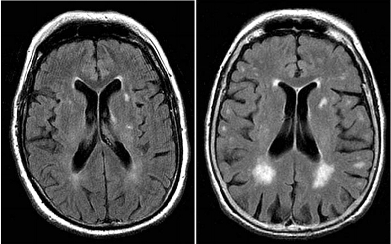
This is a description of a pratical project in machine learning at ETHZ for those that don’t have yet any significant experience in the field. It originally appeared in two parts, in the first one, I introduce you to the poject assignement. Next, I use this illustrative example to explain two important elements of the machine learning pipeline, namely preprocessing and feature extraction. In the second part, I catch up on this and give you an explanation of the remaining steps of the pipeline (model selection and validation). I then wrap up with some useful takeaways from the project, that you can eventually use in your own work and concise summary.
You’ve heard about it many times already. It is supposedly influencing how we cast our votes, putting people off their jobs and even making sure that the pineapples you buy in your supermarket are always fresh. Machine learning is a hot topic and you are increasingly likely to come across it not only in your work, but in your day to day life in general.

Warm Up
I opted for the course for several reasons, one prominent being the belief that project work can very well complement an otherwise rather theoretical course. This proved to be true and I feel I have learned a lot, also thanks to the amount of time invested in it. The project itself was divided into three parts, each of which was to be submitted at the end of following month. The project was set up as a competition and carried out in teams of three. There was in total around 130 teams taking part and competing against each other.
We were given great freedom in how to approach the problem as there was little to no guidance from the part of the instructors. One had to pick up information sort of ‘by-the-way’ during lectures or find it online. This indeed is quite an inefficient way how to get stuff done, especially if one is new in the field, but from the point of learning new concepts and acquiring useful skills, I felt that it did pretty good job. We were also allowed to implement the algorithms in a language of our choice. The most frequent choices being R, Python and Matlab. Our team opted for Python, as we all felt that getting better in it is something we will build on later. It is versatile, fun to work with, and many people, find it more than on-par with Matlab.
Data and Assignement
When one decides to tackle some problem with machine learning, arguably the first thing he must assure is access to data. The more of it he can get the better. Why? Well, imagine trying to complete a crossword puzzle that’s already half full versus a one that has only few words in it. In the former case, you can use the existing letters to support your thinking, whereas in the latter case you often need to do quite a lot of guesswork. Similarly, the more data you have as an input for your algorithm, the more confident will your final predictions be.
In the case of our project, we were provided with roughly 400 3D MRI scans of human brain. Each image is a three dimensional, 176×208×176 array of pixel values. The value of each pixel ranges from 0 to 4096 (ie. 212, corresponding to 12-bit images which are common in medical diagnostics). A slice through typical 3D image can be viewed here:
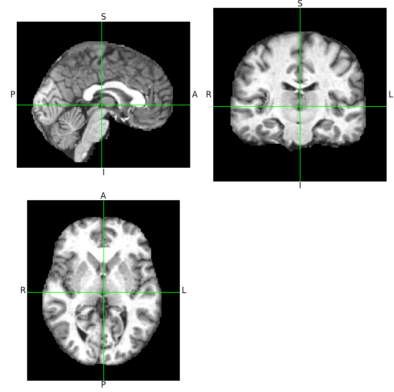
Our task in the project was divided into three parts: 1) predict person’s age, 2) predict health status and 3) predict age, health status and gender simultaneously. Together with the image data, we were provided with correct labels for 2/3 of the images. This basically means that somebody was noting the person’s age, gender and health status when taking the scan and that we were dealing with supervised learning problem. Our task then was to make prediction on remaining 1/3 of images.
Preprocessing
As a first step in practically any image analysis task, one needs to assure that the images can be easily compared against each other, that they don’t include any artifacts from the imaging process and that they contain as much useful information as possible while leaving out what we are not interested in. We call this procedure preprocessing. In the case of MRI scans, the frequent steps in this process include:
- brain extraction (removal of non-brain tissue),
- bias-field correction (compensation intensity gradients in the image that are due to magnetic field non-uniformities during scanning),
- resizing and
- voxel alignment across individual scans (voxel is a pixel in 3D space)
In our project, the available data has already been preconditioned with these approaches, thus saving us quite a lot of work that normally needs to be invested in this phase.
Feature Extraction
With good-quality input data one may proceed to arguably the most important part of a machine learning pipeline – the feature extraction. The nature of the process lies in transforming the data from a very high-dimensional space to a space with lower dimensions, while retaining the discriminative information and throwing out what will not help you in decision making.
To relate this to the task at hand, recall that initially each image represents array of more than 6 million (176×208×176) values while, at the end, you are supposed to give it a label that consists of a single number (either age or 1/0 for healthy/sick or 1/0 for male/female). The big question here is: how does one go from the former to the latter? Intuitively, not all the voxel values will play the same role in prediction. Some regions of brain will be more telling when it comes to predicting age, other when determining health status and so on. The objective in feature extraction process is to find those pixels. There are many tactics how to approach this problem. In a crude division - one can either rely on purely statistical methods, or to include so called ‘expert knowledge’.
You can better understand this with an example from the project our team was working on. Imagine having to decide whether the brain scan you are looking at belongs to a person struck by a mental illness or not. If you happen to have some knowledge on brain physiology, you may expect such disease to show up by altering the appearance of hippocampus, thus you limit your features to come only from that region. (This is what the most successful teams in this part of the project did.)
On the other hand, if you have little to no knowledge of where the “signal” should come from. then you will likely make use of some general method to disclose structure in your data. In the case of our project, we chose, arguably rather simplistic, method of histograms. One clear disadvantage of histograms you could immediately think of is that they don’t preserve spatial relationships in the data (i.e. when histogram counts pixel values, it doesn’t care about where that pixel comes from). In order to partly circumvent this, we divided the large 3D scan into 27 (3×3×3) smaller cubes and only subsequently computed histograms in each of those. In this way, we retain some, although arguably very crude, information on the distribution of pixel values in space. This is illustrated in the following image:
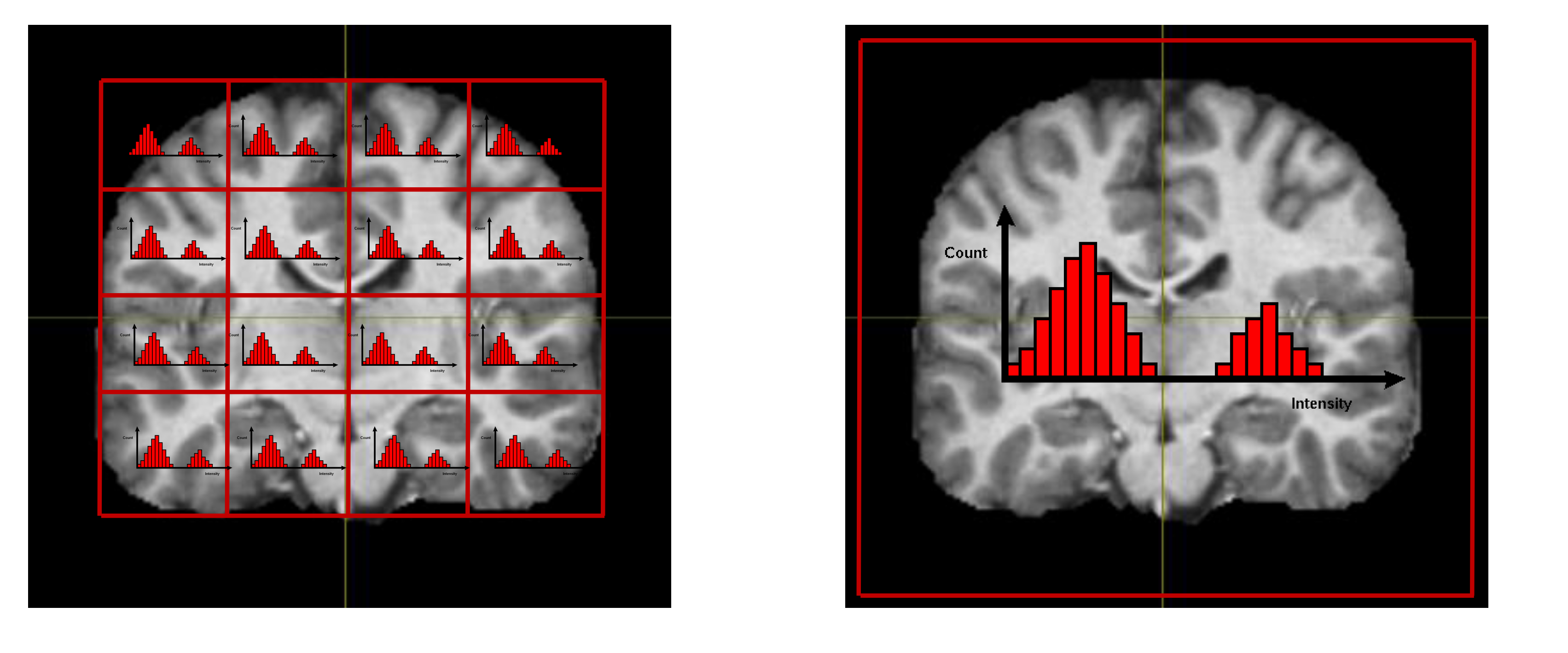
Note, that as we used 35 bins per histogram (dividing the span from 0 to 4096 into 35 equidistantly spaced intervals and counting intensity value occurrences in those), we reduced dimensionality of our problem more than 6 500× by this simple procedure.
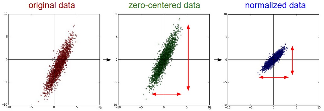
Further quasi-necessary step to be done either in the preprocessing or feature extraction stage is data conditioning. This is done mainly to improve numerical stability during subsequent steps. The common approach is to scale the data to unit variance and remove their mean, so that they are centered around zero.
Model Selection
Although we have discussed quite few steps so far, they were only preparatory (albeit necessary and crucial) and it is only now, in model selection phase, that we actually get our hands on machine learning algorithms. We can further divide this phase into two steps – training and validation. Let’s look at training first.
In the scope of our project we needed to deal with both regression and classification, here I will describe the latter one as it is perhaps more intuitive and again, I will illustrate it on an example from our project. Recalling the task at hand – to disambiguate between mentally healthy and sick patients from an MRI scan, we can imagine a simplified scenario where each brain scan is described by single two-dimensional vector of features. Further, assume that they form two point-clouds that are perfectly linearly separable as show in the figure:
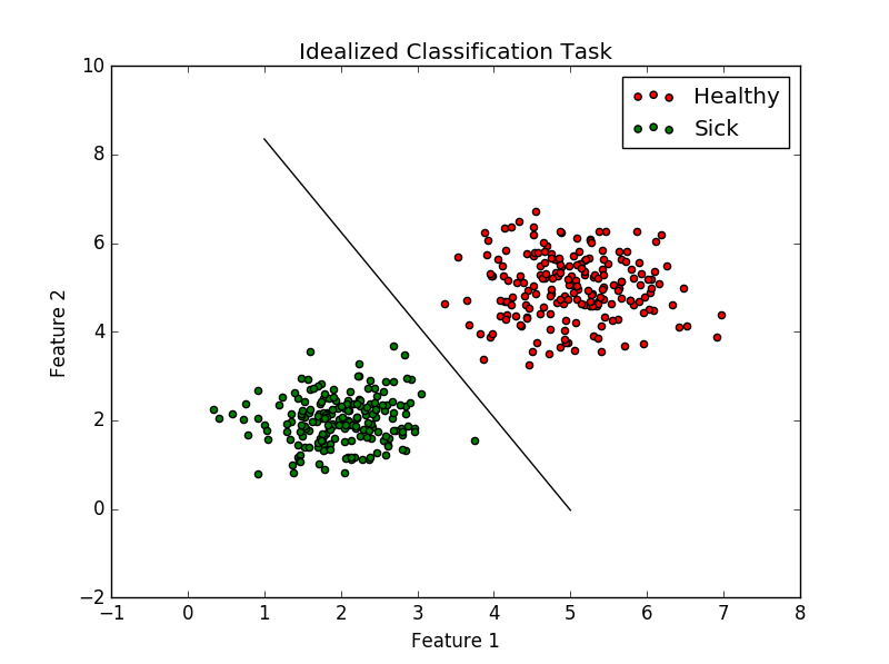
We may than write down an equation of line that divides the two-dimensional space into two half-planes. Whenever we make a new observation (take an MRI of a new patient), his brain, described by two feature vector, will fall to one of those two regions and we will label it accordingly as ‘healthy’ or ‘sick’.
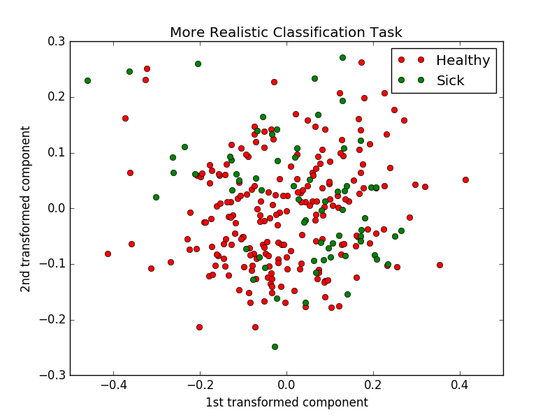
Now the situation is usually by far not that simple. First, recall that our feature vectors are n-dimensional, where n is of the order of hundreds (more precisely \(27 \times 35\ = 945\)). We may try projecting our point-clouds onto 2 dimensions, but we will likely end up with something looking like what is shown in figure above. It follows intuitively that we will have to go for something more complex than a line to separate these clusters. Nevertheless, mathematically there is no fundamental difference to how we will attempt to solve the task.
In the most general terms, proceeding with the classification example, we look for a function that, given input vector, outputs a prediction, i.e. in this case either 0 or 1, which minimizes some objective. This function is defined by set of parameters. The common objective to minimize is so called loss function which takes our prediction, true label and outputs a value that represents a penalization for misclassification. In mathematical notation, this is expressed as follows: \(\mathbf{\theta^{*}} = argmin_{\theta}\mathcal{L}(f(\textbf{X}, \mathbf{\theta}); \textbf{t}),\)
Where \(\mathbf{\theta^{*}}\) is the vector of optimal parameters, \(\mathcal{L}(\cdot)\) is a loss function, \(f(\cdot)\) is a function that gives us our prediction, \(X\) is a matrix of dimensions N×D, N and D being number of samples and features respectively, and \(t\) is a vector of true labels.
Let’s look at an example to understand this better. If the patient is healthy and we predict 0 (0 meaning no sickness), then the loss will be zero. Contrary, when we would predict 1, meaning presence of sickness, then the loss will be some nonzero value. If we take a step back and look at the problem for a while, we will easily see that we are attempting no more than function-fitting here. Of course, the number of dimensions, accessory constraints, further elements of the pipeline and the richness of the machine learning field make it rather a fancy kind of function fitting. This is nevertheless to show, that one shouldn’t expect magic to happen when confronted with machine learning algorithms. It is just math that happens to receive a lot of hype.
Validation
Let’s proceed now to the second part of model selection phase – validation. As you might have noticed, the ideal predictor function one would obtain from training phase is the one that gives 0 training loss, meaning that all samples were classified correctly. This appears desirable, but only to a point when one takes a look at decision boundaries of such a function. For illustration, let’s look how they may look like in such a case:
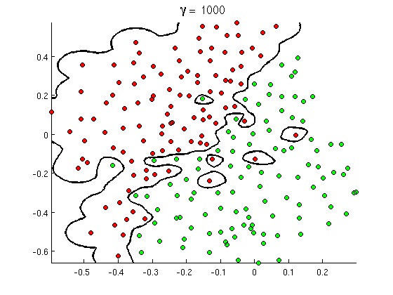
As can be seen, even if the function is optimal in a sense of giving lowest possible training loss (exactly zero as all points are classified correctly), it is by far not a good representation of the underlying structure in our data. Imagine trying to classify a new patient (ie. datapoint in this 2D plot) that falls into a region where the blue question mark is. Intuitively we would assign him among healthy patients, contrary to the, the classifier we trained will label it as sick. In other terms, the model we have obtained from training phase does poor job generalizing to new observations, we also say that we have “overfitted to training data”. It is such a prominent pitfall in machine learning that there is even an Acappella song to help you remember it and avoid it.
There are various measures one can take to address this issue. Their nature lies in estimating the generalization error of a model obtained in training phase and selection of such a model that minimizes it. Thus, one would usually define several models to be trained and then evaluate their performance on unseen samples to estimate generalization error and then opt for the one that is the most consistent, i.e. that generalizes the best. Here we come back to how useful it is to have ample data. In ideal case scenario, we would train a model on part of our dataset and evaluate it on another, that wasn’t used in training. The issue with this approach is that only rarely one has enough data to do it. This is because by holding out data from training, we arrive to a model that is too simple, we also say it has a high bias. To attenuate this, we look for approaches that put aside only small portion of samples for training from dataset. To still provide good estimate of the generalization error, we do this repeatedly and track the total error.
Let’s take a look at an example from our project again and let’s focus only on one type of a model to be trained. This still allows the situation at hand to be sufficiently complex as practically every model type is parametrized by a set of so called hyperparameters, effectively yielding whole family of models that are to be first trained and then validated. In the case of our project, and again, considering classification task, we most frequently used Support Vector Machine Classifier with Radial-basis function kernel (if you are getting lost in terminology, don’t worry, radial-basis function kernel is just a function that measures distance between points). This model has two hyperparameters, namely penalty and bandwidth (In brief these indicate how tolerant with respect to a point that gets misclassified we are and how much is our labeling of a datapoint influenced by its neighbors). We than defined range of possible values for those parameters. The rest of the job, we offloaded to off-the-shelf validation procedure GridSearchCV from scikit-learn (great Python module featuring wide array of tools for machine learning). This routine enables one to select combinations of hyperparameters and strategy for selecting samples for validation – for this we selected 10-fold cross validation (This means that in each run, model is trained on 9/10 of data and 1/10 is left out for validation. The data are reassigned after each run so that after 10 runs all samples were used exactly once for validation.)
The GridSearch routine outputs a validation error for each model it is provided with. To increase robustness (i.e. to make the model generalize better on unseen data), we ran it several times on randomly shuffled samples and calculated standard deviation among runs. As a final selection measure, we used \(mean\ error \times standard\ deviation\) among runs. The model that minimizes this metric is selected for final classification.
Results and Submission
At this point, we are basically finished with the task as described above. In the case of our project this means that we can save our predictions to a file and submit it to Kaggle (an online platform for administering big machine learning projects and competitions that hosts also university projects) to obtain a score on how well did we fare.
Although this sounds trivial, there are still some things to keep an eye on. First, the score is computed based on another portion of dataset that one isn’t allowed to access. As we are allowed to submit the solution repeatedly, it is inevitable (the less experience one has the more likely so) to try to achieve the best score. This in practice means, that there is leakage of information from the ‘hidden’ data to the model being trained. And this in turn means that we are on the best track to overfit again. This is because Kaggle uses only one half of the held-out dataset to compute the score, and usually the more we try to optimize on the available half, the worse the final score, that is based on the other half, will be. In the first two parts of the project, we made exactly this mistake, and although our predictions scored well on public leaderboard, we did poorly on the private one. For the last part of the project, we increased the robustness of model selection procedure (for example by implementing the GridSearchCV, tracking standard deviation among runs of random permutation of data, etc…) and this allowed us to perform well above average.
Remarks and Takeaway
As a final part of this post, I will share with you some tips regarding the just-described procedure. Those are the things I wish I knew at the beginning at the project, because they would save us many valuable hours. My hope is that you can make use of these tips in some of your project of your own.
- In our team, we were three people that didn’t share much classes together, this means that we didn’t get to talk to each other very often in person, which made it complicated to keep everybody on the same page and contributing more or less equally to the task. Whenever I would be to go into such a project again, I would make use of some online available task/project management tool (something we unluckily didn’t do) to track individual assignments and progress. I believe that this will make the project more enjoyable and the team more effective.
- As you could have noticed in Feature Selection section, getting good features is both crucial and sort of alchemy. One will often spend significant amount of time looking for good features and even an ample experience will usually not make this process straightforward. The recent developments in the field try to go in the opposite direction. Instead of laboriously engineering features, they consider them as part of a model to be learned. So called Convolutional Neural Networks have already outperformed the best approaches with manually designed features and thus represent attractive choices in this scenario. We haven’t used them in our project though, as for a good feature to be learned one needs to provide more than tens of thousands of images. Moreover, training of a neural network is usually very computationally expensive. One can, however, make use of some already pretrained models and then just fine-tune them for his particular task.
- We did part of our computations on cluster. As students, our submissions usually needed to wait in queue. Furthermore, once the code is evaluated, one doesn’t have access to variables created during its run. Both these facts make it time consuming to debug one’s code and try various versions of it to see which performs better. After some time, we got into practice of saving some important information during the run (like the mean errors, standard deviations, model parameters, etc..) so that we can more easily track what worked and what not. Moreover, we implemented logging routine that allows to seamlessly track progress of the code evaluation. Here I refer you to Logging Cookbook and only say that it is extremely useful tool and the extra effort of implementing pays off.
Conclusion
So that was it, you should have now an idea what happens behind the scenes when Machine Learning is referred to, what are the most important parts of the learning pipeline, what is it capable of and where some bottlenecks may be. In the scope of this post, I didn’t endeavor to go into details of the mathematical background of respective parts of the pipeline, neither did I discussed how to implement them in code. Although both very interesting, it would be out of scope of an introductory post. If you would like to find out more about the former, than I recommend you to check out some MOOCs or get a book that approaches the topic from viewpoint of statistics. If you want to find out more on how are the algorithms implemented in code, than take a look at scikit-learn documentation. Combination of both is enough to get you started exploring the richness of the machine learning on your own.
Note:
The title image is courtesy of Brain Posts blog.
comments powered by Disqus