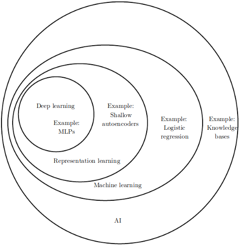
Landscape of AI
 |
 |
Artificial Intelligence: The study of intelligent agents, systems that perceive their environment and take actions that maximize their chance of successfully achieving their goals
Machine Learning: A computer program is said to learn from experience E with respect to some class of tasks T and performance measure P if its performance at tasks in T, as measured by P, improves with experience E.
Representation Learning (Feature Learning): Set of techniques that allows a system to automatically discover the representations needed for learning.
Deep Learning (Hierarchical Learning): Class of machine learning algorithms that learn multiple levels of representations that correspond to different levels of abstraction; the levels form a hierarchy of concepts.
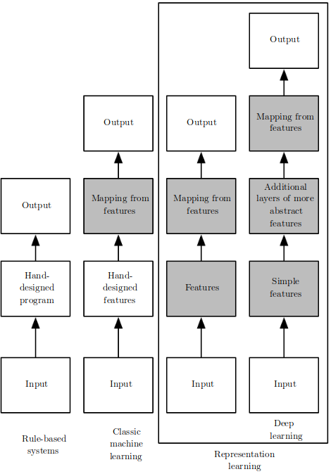
Features
 |
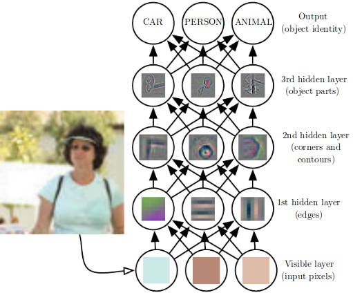 |
Expert features < deep features
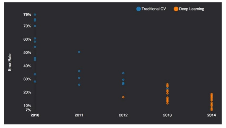
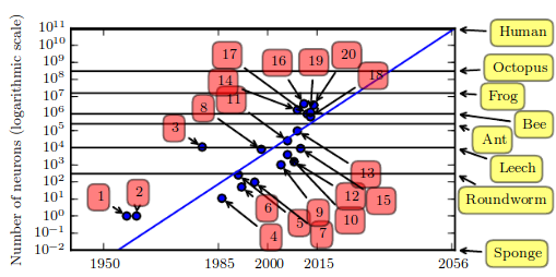
Mo' Data, Mo' GPUs
It is true that some skill is required to get good performance from a deep learning algorithm. Fortunately, the amount of skill required reduces as the amount of training data increases. The learning algorithms reaching human performance on complex tasks today are nearly identical to the learning algorithms that struggled to solve toy problems in the 1980s [...] The most important new development is that today we can provide these algorithms with the resources they need to succeed.
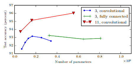
Another key reason that neural networks are wildly successful today after enjoying comparatively little success since the 1980s is that we have the computational resources to run much larger models today.
| Bigger Models | More Data |
|---|---|
 |
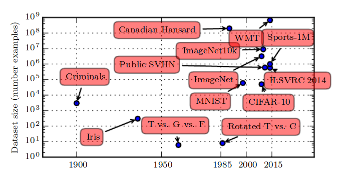 |
- As of 2016, the rule of thumb is that supervised deep learning algorithm will generally achieve acceptable performance with around 5000 examples per category and will match or exceed human performance when trained on dataset with at leas 10 million labeled examples.
Machine Learning
A computer program is said to learn from experience E with respect to some class of tasks T and performance measure P if its performance at tasks in T, as measured by P, improves with experience E.
$T$:
- Task is how ML system should process a collection of features, i.e. example $\boldsymbol{x} \in \mathbb{R}^n$
- classification (w/ or w/o missing values), regression, transcription, translation, anomaly detection, imputation, denoising, density estimation, ...
$P$:
- usually tied to the $T$
- accuracy (classification, ...), error (regression, ...), log-likelihood (density estimation, ...)
$E$:
- dataset (w/ or w/o labels)
Example: Linear Regression
$$\hat{y} = \boldsymbol{w}^T\boldsymbol{x}$$
$T$: predict $y$ from $\boldsymbol{x}$
$P$: $MSE_{test} = \frac{1}{m}\sum_i^{}(\hat{y}_i^{(test)}-y_i^{(test)})^2$
$E$: $(\boldsymbol{X}^{(train)}, \boldsymbol{y}^{(train)})$
Need: ML algorithm that improves weights $\boldsymbol{w}$ in a way that reduces $MSE_{test}$ given the training examples.
Solution: minimize $MSE_{train}$: $$\nabla_{\boldsymbol{w}} MSE_{train} = 0$$ $$ ... $$ $$\boldsymbol{w} = ({\boldsymbol{X}^{(train)}}^T\boldsymbol{X}^{(train)})^{-1}{\boldsymbol{X}^{(train)}}^T\boldsymbol{y}^{(train)}$$
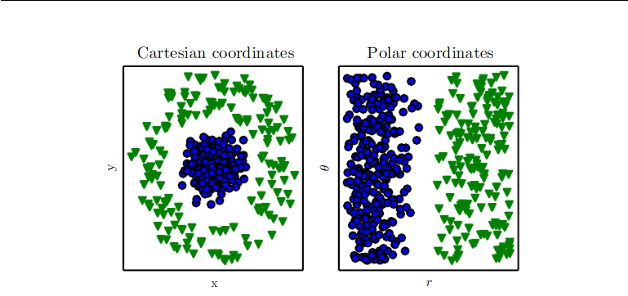
Feature Transformations
![]()
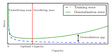
Capacity and Over-/Under- fitting
ML != Optimization ... generalization (test) error
model capacity controls whether the model is more likely to under- or over-fit
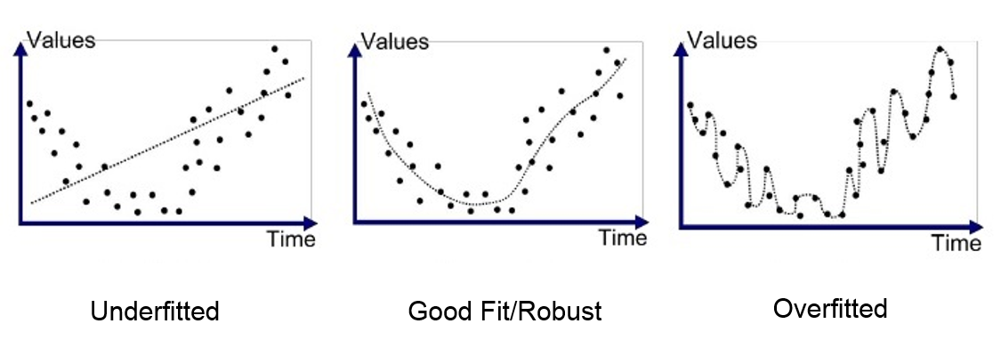
Caveat: Deep Learning models have theoretically unlimited capacity.
Occam's Razor: Among competing hypotheses that explain known observations equally well, select the "simplest" one.
Regularization
Any modification to a learning algorithm that is intended to reduce generalization error but not the training error.
E.g. penalize weights with L2 norm
$$J(\boldsymbol{w}) = MSE_{train} + \lambda\boldsymbol{w}^T\boldsymbol{w},$$
where $\lambda$ is a hyperparameter expressing our preference over possible model functions.
How to choose values of hyperparameters? -> train/validation split, e.g. 80/20
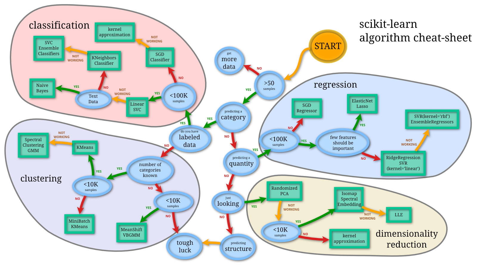
Popular ML Algorithms
Supervised:
- Linear regression, Logistic regression, LDA, SVMs, K-Nearest neighbors, Decision trees, ...
Unsupervised:
- PCA, ICA, K-Means clustering, ...
Apart from depth and width there are other considerations in terms of architecture:
- Connectivity of the layers, backward connections
- CNNs, RNNs
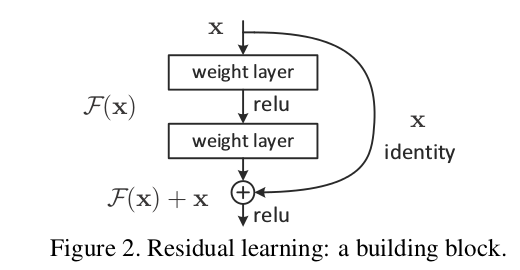
- Skip connections
- ResNets
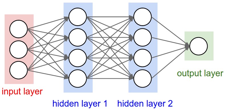
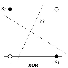
Example: Learning XOR
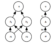
This is a toy example of deep feedforward network (also called MLP)
 |
 |
 |
$$J(\boldsymbol{\theta}) = \frac{1}{4}\sum_{\boldsymbol{x}}^{}(f(\boldsymbol{x}) - \hat{f}(\boldsymbol{x}; \boldsymbol{\theta}))^2,\quad \hat{f}(\boldsymbol{x};\boldsymbol{\theta}) = \boldsymbol{x}^T\boldsymbol{w} + b \quad \rightarrow \quad \boldsymbol{\hat{y}} = \frac{1}{2} :($$
Takeaway: Linear model can learn non-linear function via feature transformations. Instead of engineering it, you can learn it. Usually, by specifying some broader family of functions and tuning on the data.
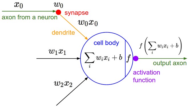
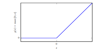
$$\boldsymbol{h}=g(\boldsymbol{W}^T\boldsymbol{x}+\boldsymbol{c}),$$ where $h$ is output of hidden unit. $$\hat{f}(\boldsymbol{x}; \boldsymbol{\theta})= \boldsymbol{w}^T \mathrm{max}\{0,\boldsymbol{W}^T\boldsymbol{x}+\boldsymbol{c}\}+b$$
Here we have used Rectified Linear Unit (ReLU) as nonlinearity $g(\cdot)$ on the hidden layer.
Solution: $$ \boldsymbol{W} = \begin{bmatrix} 1 & 1\\ 1 & 1\\ \end{bmatrix}, \qquad \boldsymbol{c} = \begin{bmatrix} 0\\ -1\\ \end{bmatrix}, \qquad \boldsymbol{w} = \begin{bmatrix} 1\\ -2\\ \end{bmatrix}, \qquad b = 0. $$
Note: There is plenty of activation functions, but ReLU is prefered.
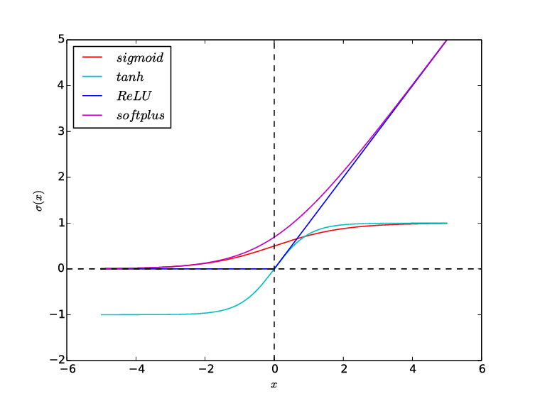
Most deep nets nowadays use ReLU for hidden layers because it avoids the vanishing gradient problem and it is faster to train than alternatives.
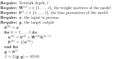
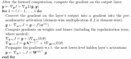
Backpropagation
Backpropagation is an algorithm that computes the chain rule of derivatives, with a specific order of computations that is highly efficient.
The derivative on each variable tells you the sensitivity of the whole expression on its value.
Chain rule
$$y=g(x) \qquad z=f(g(x))=f(y)\rightarrow \frac{dz}{dx}=\frac{dz}{dy}\frac{dy}{dz}$$
Backprop as computational graph:

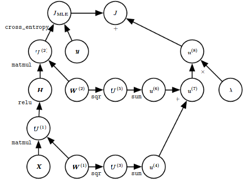
Forward Propagation for MLP as Graph
Objective:
$$J = J_{MLE} + \lambda\bigg(\sum_{i,j}^{}\big(W_{i,j}^{(1)}\big)^2 + \sum_{i,j}^{}\big(W_{i,j}^{(2)}\big)^2\bigg)$$
Regularization for DL
Deep learning algorithms are typically applied to extremely complicated domains such as images, audio sequences and text, for which the true generation process essentially involves simulating the entire universe.
What this means is that controlling the complexity of the model is not a simple matter of finding the model of the right size, with the right number of parameters. Instead, we might find - and indeed in practical deep learning scenarios, we almost always do find - that the best fitting model (in the sense of minimizing generalization error) is a large model that has been regularized appropriately.
Parameter Norm Penalties
$$\tilde{J}(\boldsymbol{\theta}; \mathbf{X},\mathbf{y}) = J(\boldsymbol{\theta};\mathbf{X},\mathbf{y}) + \lambda\Omega(\boldsymbol{\theta}),$$ express prior belief that the weights should be small and/or sparse. Constraints and Regularizers
from keras.regularizers import l1_l2
# Adds regularization term to cost function
model.add(Dense(64, input_dim=64, kernel_regularizer=l1_l2(0.2)
from keras.constraints import max_norm # l2 norm
# Directly applies scaling to weights
model.add(Dense(64, kernel_constraint=max_norm(2.)))
Sparse Representations
Express prior belief on sparse activation outputs
from keras.regularizers import l1_l2
model.add(Dense(64, input_dim=64, activity_regularizer=l1(0.2)))
Dataset Augmentation
Includes noise injection to inputs, hidden layer weights, targets. Image Preprocessing
from keras.utils import np_utils
from keras.datasets import cifar10
from keras.preprocessing.image import ImageDataGenerator

model = deep_nn() # defined elswhere

(x_train, y_train), (x_test, y_test) = cifar10.load_data()
y_train = np_utils.to_categorical(y_train, num_classes)
y_test = np_utils.to_categorical(y_test, num_classes)

datagen = ImageDataGenerator(
    featurewise_center=True,
    featurewise_std_normalization=True,
    rotation_range=20,
    width_shift_range=0.2,
    height_shift_range=0.2,
    horizontal_flip=True)

# compute quantities required for featurewise normalization
datagen.fit(x_train)

# fits the model on batches with real-time data augmentation:
model.fit_generator(datagen.flow(x_train, y_train, batch_size=32),
                    steps_per_epoch=len(x_train) / 32, epochs=epochs)
Early Stopping
Return parameters that gave the lowest validation set loss. Early Stopping
from keras.callbacks import EarlyStopping
from keras.optimizers import SGD
#define model
model = deep_nn() # this is defined elsewhere
model.compile(optimizer=SGD, loss='mse', metrics=['accuracy'])
# define early stopping callback
earlystop = EarlyStopping(monitor='val_acc', min_delta=0.0001,
                          patience=5, verbose=1, mode='auto')
callbacks_list = [earlystop]
# train the model
model_info = model.fit(train_features, train_labels,batch_size=128,
                       nb_epoch=100, callbacks=callbacks_list,
                       verbose=0,validation_split=0.2)
Parameter Sharing
Forces parameter sets to be equal.
from keras.models import Sequential
from keras.layers import Dense
from keras.layers import Embedding
from keras.layers import Conv1D,GlobalAveragePooling1D,MaxPooling1D

seq_length = 64

model = Sequential()
model.add(Conv1D(64, 3, activation='relu', input_shape=(seq_length, 100)))
model.add(Conv1D(64, 3, activation='relu'))
model.add(MaxPooling1D(3))
model.add(Conv1D(128, 3, activation='relu'))
model.add(Conv1D(128, 3, activation='relu'))
model.add(GlobalAveragePooling1D())
model.add(Dense(1, activation='sigmoid'))

model.compile(loss='binary_crossentropy', optimizer='rmsprop',
              metrics=['accuracy'])

model.fit(x_train, y_train, batch_size=16, epochs=10)
score = model.evaluate(x_test, y_test, batch_size=16)
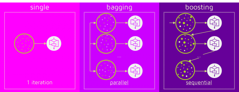
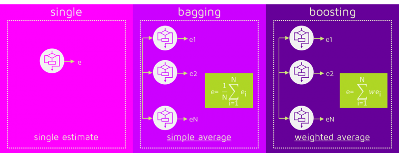
Model Averaging
Any machine learning algorithm can benefit substantially from model averaging (e.g. bagging) at the price of increased computation and memory. Machine learning competitions are usually won by methods using model averaging over dozens of models.
from sklearn.datasets import make_hastie_10_2
from sklearn.ensemble import GradientBoostingClassifier

X, y = make_hastie_10_2(random_state=0)
X_train, X_test = X[:2000], X[2000:]
y_train, y_test = y[:2000], y[2000:]

clf = GradientBoostingClassifier(n_estimators=100,learning_rate=1.0,
                                 max_depth=1, random_state=0).\
                                fit(X_train, y_train)
clf.score(X_test, y_test)
> 0.913
Check also Keras Lambda layers
Dropout
Very effective and simple regularization technique. To a first approximation, dropout is a method for making bagging practical for very many and large NNs.
from keras.models import Sequential
from keras.layers.core import Dropout, Activation
from keras.layers.convolutional import Convolution2D

model = Sequential()
model.add(Convolution2D(filters = 32, kernel_size = (8, 8),
                        strides = (4, 4), input_shape = img_size + (num_frames, )))
model.add(Activation('relu'))
model.add(Dropout(0.5))
...
"""
Vanilla Dropout
We drop and scale at train time and don't do anything at test time.
"""
p = 0.5 # prob of keeping a unit active. higher = less dropout

def train_step(X):
  # forward pass for example 3-layer neural network
  H1 = np.maximum(0, np.dot(W1, X) + b1)
  U1 = (np.random.rand(*H1.shape) < p) / p # first dropout mask.
  H1 *= U1 # drop
  H2 = np.maximum(0, np.dot(W2, H1) + b2)
  U2 = (np.random.rand(*H2.shape) < p) / p # second dropout mask.
  H2 *= U2 # drop
  out = np.dot(W3, H2) + b3

  # backward pass: compute gradients... (not shown)
  # perform parameter update... (not shown)
def predict(X):
  # ensembled forward pass
  H1 = np.maximum(0, np.dot(W1, X) + b1)
  H2 = np.maximum(0, np.dot(W2, H1) + b2)
  out = np.dot(W3, H2) + b3
Batch Normalization
Applies a transformation that maintains the mean activation close to 0 and the activation standard deviation close to 1. See docs, and be careful about batch sizes
from keras.models import Sequential
from keras.layers.core import Dropout, Activation
from keras.layers import Dense

model = Sequential()
model.add(Dense(64, input_dim=20))
model.add(BatchNormalization())
model.add(Activation('relu'))
model.add(Dropout(0.5))
...
Regularization Checkpoint:
- Use
Dropout,BatchNormalization,EarlyStoppingandl2 - Center and scale inputs, augment if possible
- Select appropriate loss function
- classification:
categorical_crossentropy,squared_hinge - regression:
huber_loss,MSE(l2 loss)
- classification:
Optimization for DL Training
Of all the many optimization problems involved in DL, the most difficult is NN training. It is quite common to invest days to months of time on hundreds of machines to solve even a single instance of the NN training problem.
Selecting Minibatch Size
- larger batches estimate gradient more accurately, but with less then linear returns
- batch should not be too small to better use hardware resources, but not too big to be able to fit to memory
- GPUs tend to prefer power 2 sized batches
Notes:
- Batches are sampled randomly
- Should shuffle the set, if data has some temporal correlation.
- Run several
epochs
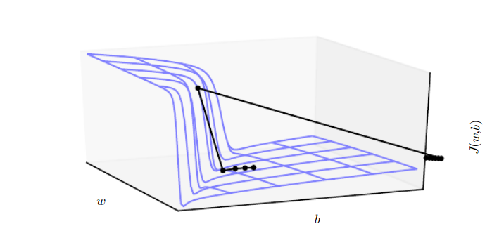
Minima, Saddles and Cliffs
Nearly any deep model is essentially guaranteed to have an extremely large number of local minima.
For many high-dimensional nonconvex functions, local minima (and maxima) are in fact rare compared to another kind of point with zero gradient: a saddle point.
- Plot norm of the gradient over time!
Gradient Clipping
clipnorm and clipvalue can be used with all optimizers
from keras import optimizers
# All parameter gradients will be clipped to:
# a maximum value of 0.5 and and a minimum value of -0.5.
sgd1 = optimizers.SGD(lr=0.01, clipvalue=0.5)
# a maximum norm of 1.
sgd2 = optimizers.SGD(lr=0.01, clipnorm=1.)
Parameter Initialization
Usually, we set the biases for each unit to heuristically chosen constants and initialize only the weights randomly.
If computational resources allow it, it is usually a good idea to treat the scale of the weights for each layer as a hyperparameter.
Optimizer Algorithms for ML
SGD, RMsprop, Adagrad, Adadelta, Adam, Adamax, Nadam
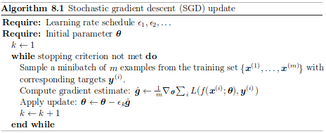
Stochastic Gradient Descent
- Classical Gradient Descent: $$w_j := w_j - \alpha \frac{\partial J(\boldsymbol{w})}{\partial w_j},$$ where $\alpha$ is learning rate, is of $\mathcal{O}(m)$
- Loss decomposes as sum over samples $$J(\boldsymbol{w}) = \frac{1}{m}\sum_i^{m}(\hat{y}_i-y_i)^2 \xrightarrow[]{\nabla_{\boldsymbol{w}}} \nabla_{\boldsymbol{w}} J(\boldsymbol{w}) = \frac{2}{m} \boldsymbol{X}^T (\boldsymbol{\hat{y}}-\boldsymbol{y})$$
- Insight: gradient is expectation that can be estimated on subset of samples
- Draw (uniformly) a fixed-sized minibatch
Adaptive Learning Rate
In practice, anneal learning rate linearly until iteration $\tau$, then keep constant: $$\epsilon_k = (1-\alpha)\epsilon_0 + \alpha\epsilon_\tau$$
from keras.optimizers import SGD
sgd = SGD(decay = 1e-6)
Momentum and Nesterov Momentum
$\theta \leftarrow \theta - \epsilon_k\hat{\boldsymbol{g}}$ becomes: $$\boldsymbol{v} \leftarrow \alpha \boldsymbol{v} - \epsilon_k\hat{\boldsymbol{g}}, \qquad \theta \leftarrow \theta + \boldsymbol{v}$$
Update step is larger if experienced gradients point consistently in one direction. Counteracts getting stopped in regions of low gradient.
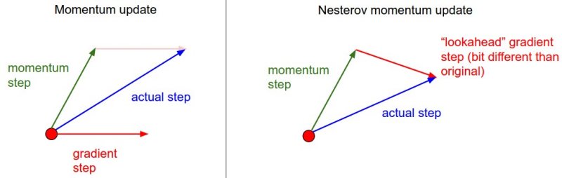
sgd = SGD(lr=0.01, decay=1e-6, momentum=0.9, nesterov=True)
Supervised Pretraining
- Train each layer separately
- Train each layer using as output of previously trained layer as input
- Train deep model, keep only $n$, $m$ layers on input and output, fill in between with randomly initialized layers to make even deeper model
Transfer Learning
- Train model on some task, keep $k$ first layers, retrain on different task (possibly with fewer samples)
Optimization for DL summary:
- Initialize layer weights from normal distribution, preferably
he_normal- or check values of gradients on single minibatch, adjust scale of initial weights accordingly
- or initialize (some) weights with supervised pretraining
- use
AdamorSGDw/ momentum - use gradient clipping
- use adaptive learning rate
- select model type according to established practice (CNNs, RNNs, ResNets, ...)
Practical Methodology (cont'd)
In practice, one can usually do much better with a correct application of a commonplace algorithm than by sloppily applying an obscure algorithm.
Recipe
- Determine your goals (performance metric and their target value)
- Establish baseline implementation of the end-to-end pipeline ASAP
- Use logging, callbacks and visualizations generously to determine bottlenecks
- Iterate with incremental changes
Performance Metrics
model.compile(loss='mean_squared_error',
              optimizer='sgd', metrics=['mae', 'acc'])
- use multiple, often problem specific
- Can report F1 score: $$F = \frac{2pr}{p+r}$$
- also Coverage, AUC
loss!=metrics
Callbacks
import numpy as np
from keras.callbacks import Callback
from keras import backend as K

def f1(y_true, y_pred):
    def recall(y_true, y_pred):

        true_positives = K.sum(K.round(K.clip(y_true * y_pred, 0, 1)))
        possible_positives = K.sum(K.round(K.clip(y_true, 0, 1)))
        recall = true_positives / (possible_positives + K.epsilon())
        return recall

    def precision(y_true, y_pred):

        true_positives = K.sum(K.round(K.clip(y_true * y_pred, 0, 1)))
        predicted_positives = K.sum(K.round(K.clip(y_pred, 0, 1)))
        precision = true_positives / (predicted_positives + K.epsilon())
        return precision

    precision = precision(y_true, y_pred)
    recall = recall(y_true, y_pred)
    return 2*((precision*recall)/(precision+recall+K.epsilon()))

class Metrics(Callback):

    def on_train_begin(self, logs={}):
        self.val_f1s = []

    def on_epoch_end(self, epoch, logs={}):
        y_pred = np.asarray(self.model.predict(\
                            self.model.validation_data[0])).round()
        y_true = self.model.validation_data[1]
        _val_f1 = f1(y_true, y_pred)
        self.val_f1s.append(_val_f1)
        return

metrics = Metrics()
...
model.fit(training_data, training_target,
          validation_data=(validation_data, validation_target),
          nb_epoch=10, batch_size=64, callbacks=[metrics])
Baseline Prototype
- Pick appropriate model (recall Occam's Razor, don't reinvent the wheel)
| Model | Feedforward | CNN | RNN |
|---|---|---|---|
| Input | fixed sized vector | topological structure | sequence |
- As a sanity check, make sure your initial loss is reasonable, and that you can achieve 100% training accuracy on a very small portion of the data
- Use available datasets and models to your advantage
- Use model ensembles for extra performance
- During training, monitor the loss, the training/validation accuracy, the magnitude of updates in relation to parameter values (it should be ~1e-3), and when dealing with ConvNets, the first-layer weights.
- Use unsupervised pre-training (domain dependent)
Additionally, use all that mentioned with Optimizers and Regularization
Do I need more data?
Many ML novices are tempted to make improvements by trying out many different algorithms. Yet, it is often much better to gather more data than to improve the learning algorithm.
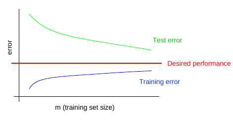
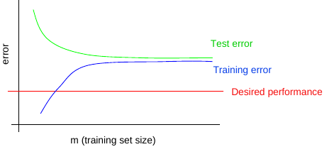
- performance on training set poor => more data won't help
- test set performance poor & train set performance good => get more data
How much data do I need?
Usually, adding a small fraction of the total number of examples will not have noticeable on generalization error. As a rule of thumb, aim at least at doubling the training set size.
Selecting hyperparameters
Manual vs. Automatic
If you have time to tune only one hyperparameter, tune the learning rate.
NN can sometimes perform well with only a small number of tuned hyperparameters, but often benefit significantly from tuning forty or more.
Random Search > Grid Search
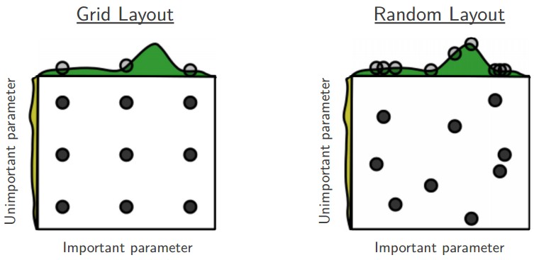
Example: $$\texttt{log_learning_rate} \tilde{} U(-1, -5),$$ $$\texttt{learning_rate} = 10^{\texttt{log_learning_rate}}$$
Debugging Strategies for ML
Machine learning systems are difficult to debug [...]

- Visualize model in action
- Visualize the worst mistakes
- Check training and test errors
- Bias / Variance trade-off
- Fit a tiny dataset
- Monitor histograms of activations and gradients
- Prototype, fail & improve
| High Variance (overfit) | High Bias (bad/few features) |
|---|---|
 |
 |
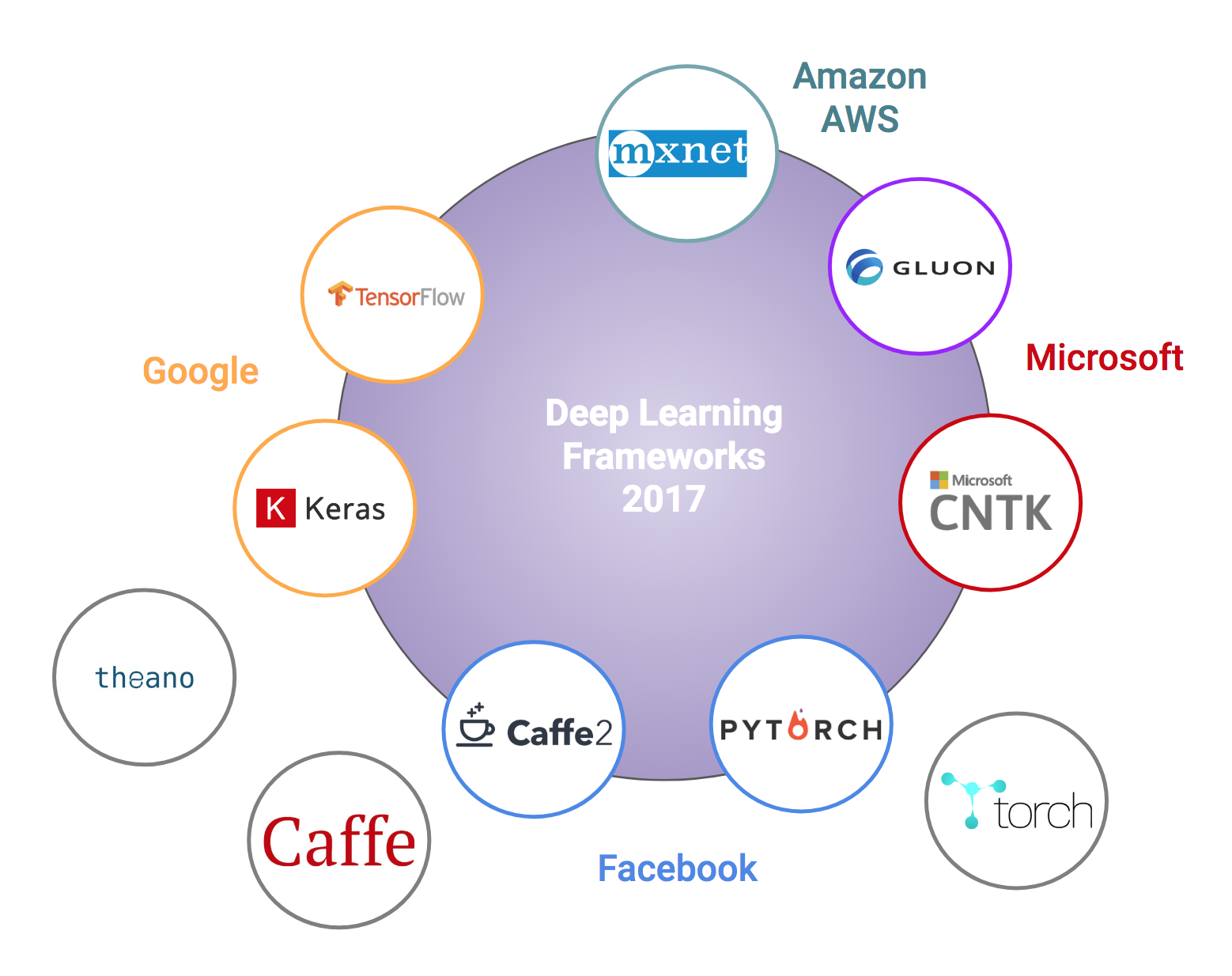
Frameworks for DL
Summary
(out all of this, what you should remember)
General:
- Good features need good resources
- Callbacks, logging and visualizations are must from very start
- Use existing data and models to your advantage
- Building models with
kerasis easy
Regularization:
- Use
Dropout,BatchNormalization,EarlyStoppingandl2 - Center and scale inputs, augment if possible
- Select appropriate loss function (
categorical_crossentropy,huber_loss, ...)
Optimization:
- use
AdamorSGDw/ momentum; gradient clipping; adaptive lr - initialize weights properly
References
- http://www.deeplearningbook.org/
- http://cs229.stanford.edu/materials/ML-advice.pdf
- http://cs231n.github.io
Reading
- http://blog.dennybritz.com/2017/01/17/engineering-is-the-bottleneck-in-deep-learning-research/
- https://developers.google.com/machine-learning/rules-of-ml/
- https://becominghuman.ai/cheat-sheets-for-ai-neural-networks-machine-learning-deep-learning-big-data-678c51b4b463
- http://web.mit.edu/16.070/www/lecture/big_o.pdf
- https://www.tensorflow.org/versions/r1.0/get_started/summaries_and_tensorboard
- https://anvaka.github.io/rules-of-ml/
- https://databricks.com/session/deep-learning-with-apache-spark-and-gpus
- deeplearning-biology
- awesome-deepbio
- https://github.com/tensorflow/models
Neural Network - MWE
# Imports
import numpy as np

from sklearn.model_selection import train_test_split
from sklearn.linear_model import LogisticRegressionCV
from sklearn.datasets import load_iris

from keras.models import Sequential
from keras.layers import Dense, Activation, Dropout, BatchNormalization
from keras.utils import np_utils

# One hot encoding
def one_hot_encode_object_array(arr):
    '''One hot encode a numpy array of objects (e.g. strings)'''
    uniques, ids = np.unique(arr, return_inverse=True)
    return np_utils.to_categorical(ids, len(uniques))

train_y_ohe = one_hot_encode_object_array(train_y)
test_y_ohe = one_hot_encode_object_array(test_y)
# Logistic Regression
iris = load_iris()
X = iris["data"]
y = iris["target"]
train_X, test_X, train_y, test_y = \
    train_test_split(X, y, train_size=0.6, test_size=0.4,
                     shuffle=True, random_state=0)
lr = LogisticRegressionCV()
lr.fit(train_X, train_y)
print("Accuracy = {:.2f}".format(lr.score(test_X, test_y)))
# Toy Feedforward net
model = Sequential()

model.add(Dense(16, input_shape=(4,)))
model.add(Activation('relu'))

model.add(Dense(3))
model.add(Activation('softmax'))

model.compile(optimizer='adam',
              loss='categorical_crossentropy', metrics=["accuracy"])
model.fit(train_X, train_y_ohe, epochs=100, batch_size=1, verbose=0)

loss, accuracy = model.evaluate(test_X, test_y_ohe, verbose=0)
print("Accuracy = {:.2f}".format(accuracy))
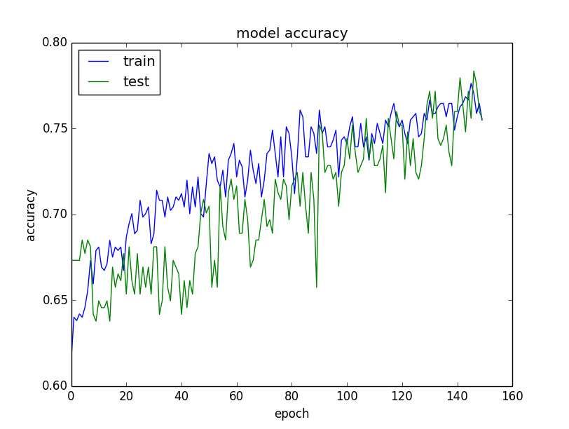
Important! This is super simplistic, normally you should include the recommended regularizers, optimization settings, callbacks, visualizations, ...
We have likely overfitted
# Report Settings
from keras import __version__ as K_ver
from keras.backend import _config as K_cf
from tensorflow import __version__ as tf_ver
print("Tensorflow version: {}".format(tf_ver))
print("Keras version: {}".format(K_ver))
print("Keras config: {}".format(K_cf))
Tensorboard Example
| Accuracy | Cost |
|---|---|
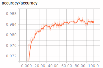 |
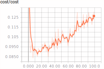 |